Homework 2: Empirical Risk and Simple Linear Regression

due Wednesday, May 13th, 2026 at 11:59PM Ann Arbor Time

Write your solutions to the following problems either by writing them on a piece of paper or on a tablet and scanning your answers as a PDF. Note that you are not allowed to use LaTeX, Google Docs, or any other digital document creation software to type your answers. Homeworks are due to Gradescope by 11:59PM on the due date. See the syllabus for details on the slip day policy.

Homework will be evaluated not only on the correctness of your answers, but on your ability to present your ideas clearly and logically. You should always explain and justify your conclusions, using sound reasoning. Your goal should be to convince the reader of your assertions. If a question does not require explanation, it will be explicitly stated.

Before proceeding, make sure you’re familiar with the collaboration policy.

Total Points: 10 + 7 + 9 + 8 + 9 + 9 = 52

Problem 1: Homework 1 Solutions Review (10 pts)

Review the solutions to Homework 1. Pick two problem parts (for example, Problem 3a and Problem 5) from Homework 1 in which your solutions have the most room for improvement, i.e., where they have unsound reasoning, could be significantly more efficient or clearer, etc. Include a screenshot of your solution to each problem part, and in a few sentences, explain what was deficient and how it could be fixed.

Alternatively, if you think one of your solutions is significantly better than the posted one, copy it here and explain why you think it is better. If you didn’t do Homework 1, choose two problem parts from it that look challenging to you, and in a few sentences, explain the key ideas behind their solutions in your own words.

Problem 2: Stonks (7 pts)

This problem will eventually have something to do with machine learning. But first, a life lesson.

Suppose you invest in a stock, and:

In year 1, your investment increases by 50%.
In year 2, your investment decreases by 50%.
In year 3, your investment increases by 50%.
In year 4, your investment decreases by 50%.

What is the average growth rate of your investment, per year? The answer is not 0%, because ultimately you’ve lost money, even though it looks like the gains and losses should cancel out.

Why? At end of year 1, you have more money than you started with, and so losing 50% of that money in year 2 hurts more than losing 50% of your starting amount. Then, going up 50% in year 3 earns you less money than originally going up 50% in year 1 did, and so on.

Before we calculate the average growth rate, let’s calculate the final value of your investment. To do so, we should convert these growth rates from percentages multipliers, using the formula:

\text{multiplier} = 1 + \frac{\text{percentage}}{100}

So,

\text{final value} = \text{initial value} \cdot \underbrace{1.5}_{\text{year } 1} \cdot \underbrace{0.5}_{\text{year } 2} \cdot \underbrace{1.5}_{\text{year } 3} \cdot \underbrace{0.5}_{\text{year } 4} = \text{initial value} \cdot 0.5625

Converting $$0.5625$$ from a percentage back to a growth rate gives us:

\text{percentage} = 0.5625 - 1 = -0.4375 = -43.75\%

So, in total, we lost 43.75% of our money.

This doesn’t give us our average growth rate, though. The average growth rate, as a multiplier, should be a value $$g$$ such that if our investment grows by $$g$$ each year, we end up with $1.5 \cdot 0.5 \cdot 1.5 \cdot 0.5 \cdot \text{initial value}$ . In other words:

\text{final value} = \text{initial value} \cdot g^4

So, as a multiplier, we have that:

g^4 = 1.5 \cdot 0.5 \cdot 1.5 \cdot 0.5 \implies g = \left( 1.5 \cdot 0.5 \cdot 1.5 \cdot 0.5 \right)^{1/4} \approx 0.8660

Converting $$g$$ back to a percentage gives us:

\text{percentage} = 0.8660 - 1 = -0.1340 = -13.40\%

So, the average growth rate of our investment, per year, is $-13.40\%$ — not the 0% that we might initially guess.

What does this have to do with machine learning? Let’s re-visit one particular calculation above.

g = \left( 1.5 \cdot 0.5 \cdot 1.5 \cdot 0.5 \right)^{1/4}

Here, $$g$$ , is the geometric mean of the numbers 1.5, 0.5, 1.5, and 0.5. Geometric means are useful in computing the average of growth rates (when expressed as multipliers). In general, if $y_1, y_2, \ldots, y_n$ are positive numbers, then their geometric mean is:

\left(y_1 \cdot y_2 \cdot \ldots \cdot y_n\right)^{1/n} = \left(\prod_{i=1}^n y_i\right)^{1/n}

Like the arithmetic mean, as we saw in Chapter 1.2, and the harmonic mean, as we saw in Lab 2, the geometric mean is the constant prediction that minimizes average loss for some loss function.

In this case, the loss function is the log-quotient loss, defined as:

\begin{aligned} L_{LQ}(y_i, h(x_i)) &= \left[\log\left(\frac{y_i}{h(x_i)}\right)\right]^2 \end{aligned}

Note that $\log(\cdot)$ is the natural logarithm, with base $$e$$ .

Prove that the geometric mean of $y_1, y_2, \ldots, y_n$ is the constant prediction that minimizes average log-quotient loss for the constant model, i.e. that the geometric mean minimizes:

R_{LQ}(w) = \frac{1}{n} \sum_{i=1}^n \left[\log\left(\frac{y_i}{w}\right)\right]^2

Hint: As in Lecture 3, you’ll want to start by finding $\frac{\text{d}}{\text{d}w} R_{LQ}(w)$ and setting that to 0. As a sub-problem, you’ll need to find $\frac{\text{d}}{\text{d}w} \left[\log\left(\frac{y_i}{w}\right)\right]$ . Work one step at a time and make sure your logic is clearly justified. Review the logarithm rules presented in Homework 1, Problem 5, and also use the fact that if $b = \log(a)$ , then $$a = e^b$$ .

Problem 3: Pythagorean Means (7 pts)

In Problem 1, you discovered the geometric mean, and saw that it’s useful in computing the average of growth rates. In Labs 1 and 2, you discovered the harmonic mean, and saw that it’s useful to compute the average of rates, like speeds. The geometric mean, harmonic mean, and the “regular” arithmetic mean are collectively known as “Pythagorean means”.

For an arbitrary dataset of positive numbers $y_1, \ldots, y_n$ , they are defined as follows:

Arithmetic mean: $\displaystyle \frac{1}{n} \sum_{i=1}^n y_i$
Geometric mean: $\displaystyle \left( \prod_{i=1}^n y_i \right)^{1/n}$
Harmonic mean: $\displaystyle \frac{n}{\sum_{i=1}^n \frac{1}{y_i}}$

(3 pts) For the following dataset, compute all three of the means defined above.

$$ 1, 2, 2, 4, 8 $$

Then, think about why the definitions of the geometric and harmonic means require the numbers to be positive. (You don’t need to write your answer anywhere.)

(4 pts) In the above example, you may have noticed that:

\text{arithmetic mean} \geq \text{geometric mean} \geq \text{harmonic mean}

This inequality is true in general, for any dataset of positive numbers $y_1, \ldots, y_n$ . This is known as the AM-GM-HM inequality.

Use the fact that the AM-GM inequality holds true to prove the GM-HM inequality. That is, given that:

\frac{1}{n} \sum_{i=1}^n y_i \geq \left( \prod_{i=1}^n y_i \right)^{1/n}

Prove that:

\left( \prod_{i=1}^n y_i \right)^{1/n} \geq \frac{n}{\sum_{i=1}^n \frac{1}{y_i}}

Hint: Start by assuming the AM-GM inequality holds true, and define $z_i = \frac{1}{y_i}$ . Then, try and re-write the right side of the inequality to look like $\frac{1}{n} \sum_{i=1}^n z_i$ .

If you’re curious, read more about the history of the Pythagorean means here. These means were developed by the followers of ancient mathematician Pythagoras (whose namesake theorem you’re familiar with) in the context of understanding harmonies in music. And you now know how to derive each one by minimizing average loss for the constant model, each one through a different loss function!

Problem 4: Slippery Slope (9 pts)

In Chapter 1.3, we found that $w^* = \mathrm{Median}(y_1, y_2, \ldots, y_n)$ is the constant prediction that minimizes mean absolute error:

R_{\mathrm{abs}}(w) = \frac{1}{n} \sum_{i=1}^n |y_i - w|

Suppose that we have a dataset of numbers $y_1, y_2, \ldots, y_n$ such that $$n$$ is odd and the values are arranged in increasing order. That is, $y_1 \leq y_2 \leq \cdots \leq y_n$ .

Note: Parts a) and b) are independent of each other.

(5 pts) Suppose that $R_{\mathrm{abs}}(\alpha) = V$ , where $$V$$ is the minimum value of $R_{\mathrm{abs}}(w)$ and $\alpha$ is one of the numbers in our dataset.

Let $\alpha + \beta$ be the smallest value greater than $\alpha$ in our dataset, where $\beta > 0$ . Another way of thinking about this is that $\beta =$ (smallest value greater than $\alpha$ ) $- \alpha$ .

Suppose we modify our dataset by replacing the value $\alpha$ with the value $\alpha + \beta + 1$ . In our new dataset of $$n$$ values:

What value of $$w$$ minimizes $R_{\mathrm{abs}}(w)$ ?
What is the new minimum value of $R_{\mathrm{abs}}(w)$ ?

Both of your answers should be expressions involving $$V$$ , $\alpha$ , $\beta$ , and/or constants.

(4 pts) Let $$y_a$$ and $$y_b$$ be two values in our dataset such that $$y_a < y_b$$ and that the slope of $R_{\mathrm{abs}}(w)$ between $$w = y_a$$ and $$w = y_b$$ is constant, and equal to $-\frac{2}{3}$ .

Suppose we introduce a new value to our dataset that is less than $$y_a$$ . In our new dataset of $$n+1$$ values, what is the slope of $R_{\mathrm{abs}}(w)$ between $$w = y_a$$ and $$w = y_b$$ ? Your answer should be an expression involving $$n$$ and/or constants, but should not contain $$a$$ or $$b$$ , or any value of $$y$$ .

Problem 5: Fun with Correlation (8 pts)

As we saw in Chapter 1.4, the correlation coefficient $$r$$ between two variables $$x$$ and $$y$$ measures the strength of the linear association between them, or intuitively, how tightly the points cluster around a line. Formally, $$r$$ is defined as:

r = \frac{1}{n} \sum_{i=1}^n \left( \frac{x_i - \bar{x}}{\sigma_x} \right) \left( \frac{y_i - \bar{y}}{\sigma_y} \right)

where $\bar{x}$ and $\bar{y}$ are the means of $$x$$ and $$y$$ , respectively, and $\sigma_x$ and $\sigma_y$ are the standard deviations of $$x$$ and $$y$$ , respectively.

(3 pts) Let $$r$$ be the correlation coefficient between $$x$$ and $$y$$ . Let $$z$$ be a new variable defined as:

z_i = -2x_i + 5, \qquad i = 1, \ldots, n

Let $$r’$$ be the correlation coefficient between $$z$$ and $$y$$ . Prove that $$r’ = -r$$ .

Hint: You can use the facts that if $$z_i = ax_i + b$$ , then $\bar{z} = a\bar{x} + b$ and $\sigma_z = |a|\sigma_x$ , without proof. Everything else must be derived from the definition of the correlation coefficient.

(5 pts) Suppose we fit two simple linear regression models by minimizing mean squared error.

Model 1: $\text{predicted } y_i = h(x_i) = w_0^* + w_1^* x_i$
Model 2: $\text{predicted } y_i = h’(z_i) = w_0’ + w_1’ z_i$

(The $$‘$$ does not indicate a derivative here!)

We already know that $$r’ = -r$$ . How do the other quantities compare between the two lines?

Express $$w_1’$$ in terms of $$w_1^*$$ , $$w_0^*$$ , and/or constants (but no other variables).
Express $$w_0’$$ in terms of $$w_0^*$$ , $$w_1^*$$ , and/or constants (but no other variables).
Above, you should have found that the new slope, $$w_1’$$ , and new intercept, $$w_0’$$ , are different than the original slope and intercept. However, it turns out that the mean squared error of both model’s predictions are the same. That is:

\frac{1}{n} \sum_{i=1}^n (y_i - (w_0' + w_1' z_i))^2 = \frac{1}{n} \sum_{i=1}^n (y_i - (w_0^* + w_1^* x_i))^2

Give a two-sentence English explanation of why this is the case.

(0 pts, optional) This part is challenging and potentially time-consuming, so we’ve made it optional. It’s good exam practice though, so if you don’t do it now, you should return to it later on when you have more time. It is independent of the previous two parts of this problem.

Prove that, for any dataset $(x_1, y_1), \ldots, (x_n, y_n)$ with a correlation coefficient $$r$$ ,

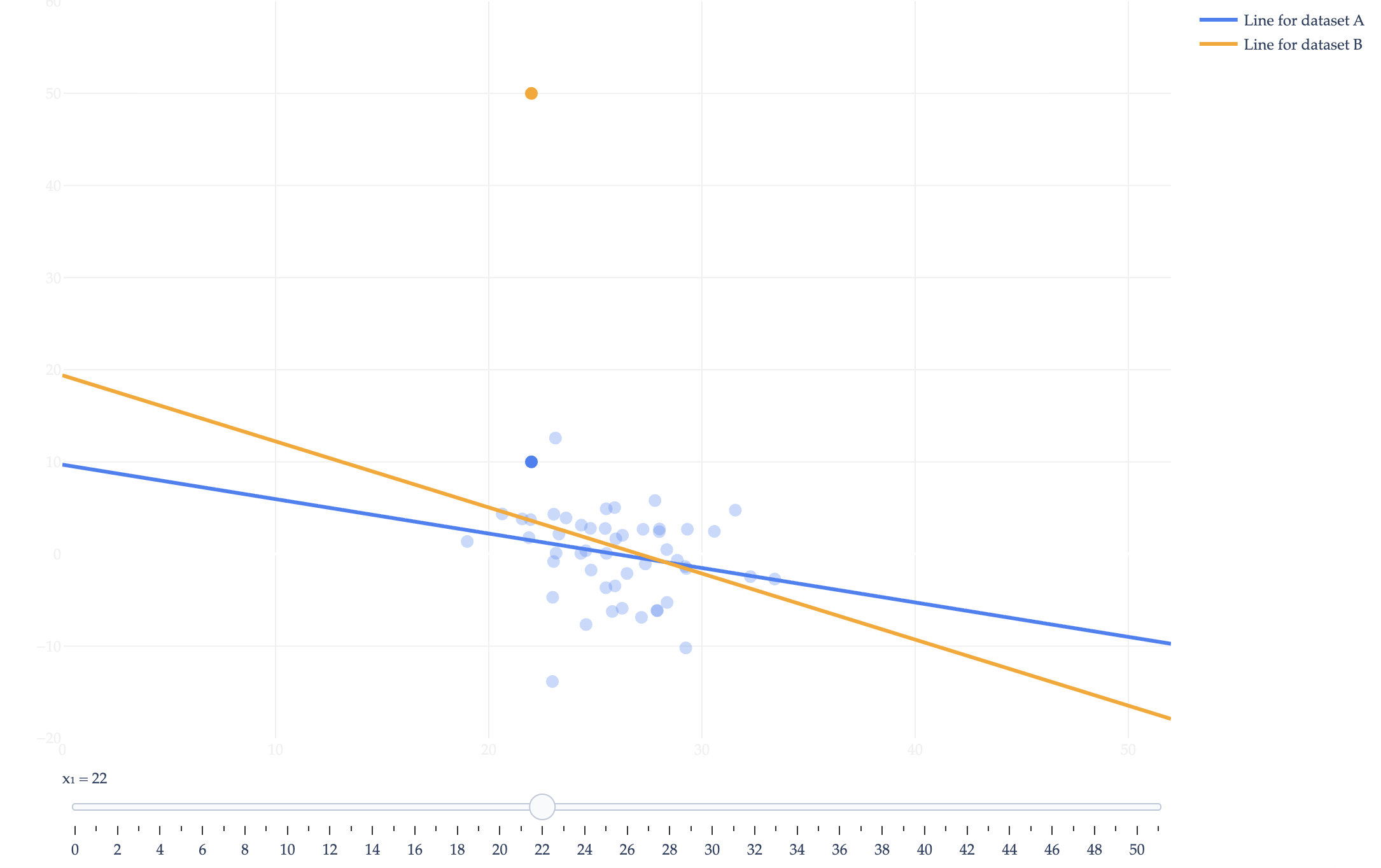
\underbrace{\frac{1}{n} \sum_{i=1}^n (y_i - (w_0^* + w_1^* x_i))^2}_{\text{mean squared error of optimal SLR model}} = \underbrace{\sigma_y^2 (1 - r^2)}_{\text{function of correlation coefficient}}

Problem 6: Switching Sides (9 pts)

Consider two datasets, $$A$$ and $$B$$ . Both datasets have $$n = 50$$ points, of which 49 are identical, and only one is different between the two datasets:

Dataset $$A$$ : $(26, 10), (x_2, y_2), \ldots, (x_{49}, y_{49}), (x_{50}, y_{50})$
Dataset $$B$$ : $(26, 50), \underbrace{(x_2, y_2), \ldots, (x_{49}, y_{49}), (x_{50}, y_{50})}_{\text{identical in both datasets}}$

Suppose that in both datasets, the $$x$$ -values have a mean of $\bar{x} = 26$ and a standard deviation of $\sigma_x = \sqrt{\frac{1}{n} \sum_{i=1}^n (x_i - \bar{x})^2} = 3$ .

(4 pts) Suppose we fit a simple linear regression model by minimizing mean squared error, separately for each dataset.

Let $$w_1^A$$ and $$w_1^B$$ be the optimal slopes for datasets $$A$$ and $$B$$ , respectively. Determine the difference between $$w_1^B$$ and $$w_1^A$$ . That is, find:

$$ w_1^B - w_1^A $$

Your answer should be a number with no variables.

Hint: There are many equivalent formulas for the slope of the regression line. We recommend using this one for this problem:

w_1^* = \displaystyle\frac{\displaystyle\sum_{i=1}^n (x_i - \overline x)y_i}{\displaystyle\sum_{i=1}^n (x_i - \overline x)^2}

(3 pts) Let $$h_A$$ and $$h_B$$ be the simple linear regression lines for datasets $$A$$ and $$B$$ , respectively. That is, $$h_A(x_i) = w_0^A + w_1^A x_i$$ and $$h_B(x_i) = w_0^B + w_1^B x_i$$ .

Which of the following values is greater: $$|h_A(43) - h_B(43)|$$ or $$|h_A(24) - h_B(24)|$$ ? Why?

Hint: Intuitively, we’re asking which input’s predicted value changes more by switching from $$A$$ to $$B$$ . Don’t try and expand the absolute differences or find their values exactly. Instead, draw a picture of both lines. For each line, there is one point that it is guaranteed to pass through. Using your knowledge of that point, and the slopes of the lines, you should be able to reason about which difference is greater.

(2 pts) When initially writing this problem, we gave it a real-world theme involving athletes and their salaries. However, we decided that the story made the problem too long, and made it more difficult to understand the relevant ideas. But, you may feel that the resulting problem seemed too abstract.

Would you have preferred a real-world theme in this problem, or do you prefer the simplified, straight-forward version, and why? (As long as you provide an answer and a reason, you’ll receive full credit. There is no right answer.)

Problem 7: Simple LAD (9 pts)

This problem involves writing code and submitting it to the Gradescope autograder.

There are two ways to access the supplemental Jupyter Notebook:

Option 1: Click here to open hw02.ipynb on DataHub. Before doing so, read the instructions on the Tech Support page on how to use the DataHub.
Option 2: Set up a Jupyter Notebook environment locally, use git to clone our course repository, and open homeworks/hw02/hw02.ipynb. For instructions on how to do this, see the Tech Support page of the course website.

To receive credit for the programming portion of the homework, you’ll need to submit your completed notebook to the autograder on Gradescope. Your submission time for Homework 2 is the latter of your PDF and code submission times.