Lab 2: Empirical Risk and Simple Linear Regression

due for completion at 11:59PM Ann Arbor Time on Monday, May 11th, 2026

Each lab worksheet will contain several activities, some of which will involve writing code and others that will involve writing math on paper. To receive credit for a lab, you must complete as many of the activities as you can in 2 hours and submit a PDF of your work to Gradescope. We will provide specific instructions on how to submit programming activities (e.g. submitting the notebook or including a screenshot of some output).

Feel free to work with others in the course, but you must submit individually.

Activities

Activity 1: Relative Squared Loss
Activity 2: Rapid Fire
Activity 3: Slope of Mean Absolute Error
Activity 4: Programming
Activity 5: Reverse Regression
Activity 6: Transformed Data
Activity 7: Relative Squared Loss, Continued
Activity 8: The Meaning of Mean Squared Error
Activity 9: What Do You Mean?
Activity 10: A Refresher

Recap: The Modeling Recipe

In Chapter 1.3, we introduced the three-step modeling recipe for finding optimal model parameters, which ultimately helps us make the best possible predictions.

Choose a model.

\underbrace{h(x_i) = w}_{\text{constant model}} \quad\quad \underbrace{h(x_i) = w_0 + w_1 x_i}_{\text{simple linear regression model}}

Choose a loss function.

\underbrace{L_{\text{sq}}(y_i, h(x_i)) = (y_i - h(x_i))^2}_{\text{squared loss}} \quad\quad \underbrace{L_{\text{abs}}(y_i, h(x_i)) = |y_i - h(x_i)|}_{\text{absolute loss}}

Minimize average loss (also called empirical risk) to find optimal model parameters.
- Constant model, squared loss: $\displaystyle R_{\text{sq}}(w) = \frac{1}{n} \sum_{i=1}^n (y_i - w)^2 \implies w^* = \bar{y}$
- Constant model, absolute loss: $\displaystyle R_{\text{abs}}(w) = \frac{1}{n} \sum_{i=1}^n |y_i - w| \implies w^* = \text{Median}(y_1, y_2, \ldots, y_n)$
- Simple linear regression model, squared loss:

\displaystyle R_{\text{sq}}(w_0, w_1) = \frac{1}{n} \sum_{i=1}^n (y_i - (w_0 + w_1 x_i))^2 \implies w_1^* = \frac{\sum_{i=1}^n (x_i - \bar{x})(y_i - \bar{y})}{\sum_{i=1}^n (x_i - \bar{x})^2}, \quad w_0^* = \bar{y} - w_1^* \bar{x}

Activity 1: Relative Squared Loss

Suppose we’d like to find the optimal parameter, $$w^*$$ , for the constant model $$h(x_i) = w$$ . To do so, we use the following loss function, called the relative squared loss:

L_{\text{rsq}}(y_i, h(x_i)) = \frac{(y_i - h(x_i))^2}{y_i}

What value of $$w$$ minimizes the average loss (i.e. empirical risk) when using the relative squared loss function – that is, what is $$w^*$$ ? Your answer should only be in terms of the variables $n, y_1, y_2, \ldots, y_n$ , and any constants.

Solution

Since $$h(x_i) = w$$ for the constant model, relative squared loss for the constant model is:

L_{\text{rsq}}(y_i, w) = \frac{(y_i - w)^2}{y_i}

and so average relative squared loss for the constant model is:

R_{\text{rsq}}(w) = \frac{1}{n} \sum_{i = 1}^n \frac{(y_i - w)^2}{y_i}

To find the value of $$w$$ that minimizes $R_{\text{rsq}}(w)$ , we’ll first find its first derivative and set it to zero. The first derivative of $R_{\text{rsq}}(w)$ is:

\begin{align*} \frac{\text{d}}{\text{d} w} R_{\text{rsq}}(w) &= \frac{\text{d}}{\text{d} w} \left( \frac{1}{n} \sum_{i = 1}^n \frac{(y_i - w)^2}{y_i} \right) \\\\ &= \frac{1}{n} \sum_{i = 1}^n \frac{\text{d}}{\text{d} w} \left( \frac{(y_i - w)^2}{y_i} \right) \\\\ \end{align*}

At this point, it’ll be useful to step aside and find the derivative of $L_{\text{rsq}}(y_i, w)$ with respect to $$w$$ , as this is the expression being summed. The derivative of $L_{\text{rsq}}(y_i, w)$ with respect to $$w$$ is:

\begin{align*} \frac{\text{d}}{\text{d}w} L_{\text{rsq}}(y_i, w) &= \frac{\text{d}}{\text{d}w} \frac{(y_i - w)^2}{y_i} \\\\ &= \frac{1}{y_i} \cdot \frac{\text{d}}{\text{d}w} (y_i-w)^2 \\\\ &= \frac{1}{y_i} \cdot 2 (y_i-w) \cdot (-1) \\\\ &= -2 \cdot \frac{y_i-w}{y_i} \\\\ &= \boxed{2\cdot \frac{w}{y_i} -2} \end{align*}

Back to $\frac{\text{d}}{\text{d} w}R_{\text{rsq}}(w)$ , we have:

\begin{align*} \frac{\text{d}}{\text{d} w} R_{\text{rsq}}(w) &= \frac{1}{n} \sum_{i = 1}^n \frac{\text{d}}{\text{d} w} \left( \frac{(y_i - w)^2}{y_i} \right) \\\\ &= \frac{1}{n} \sum_{i = 1}^n \left( 2\cdot \frac{w}{y_i} -2 \right) \\\\ &= \frac{2w}{n} \sum_{i=1}^n (\frac{1}{y_i}) - \frac{1}{n} \sum_{i=1}^n 2 \\\\ &= \frac{2w}{n} \sum_{i=1}^n (\frac{1}{y_i}) - 2 \end{align*}

Setting this equal to 0 yields:

\begin{align*} \frac{2w}{n} \sum_{i=1}^n (\frac{1}{y_i}) - 2 &= 0 \\\\ \frac{w}{n} \sum_{i=1}^n (\frac{1}{y_i}) &= 1 \\\\ w^* &= \frac{1}{\frac{1}{n} \sum_{i=1}^n (\frac{1}{y_i})} \\\\ w^* &= \boxed{\frac{n}{\sum_{i=1}^n \frac{1}{y_i}}} \\\\ \end{align*}

This is known as the harmonic mean of $$y_1, y_2, \dots, y_n$$ .

Activity 2: Rapid Fire

Consider a dataset of $$n$$ integers, $y_1, y_2, \ldots, y_n$ , whose histogram is given below:

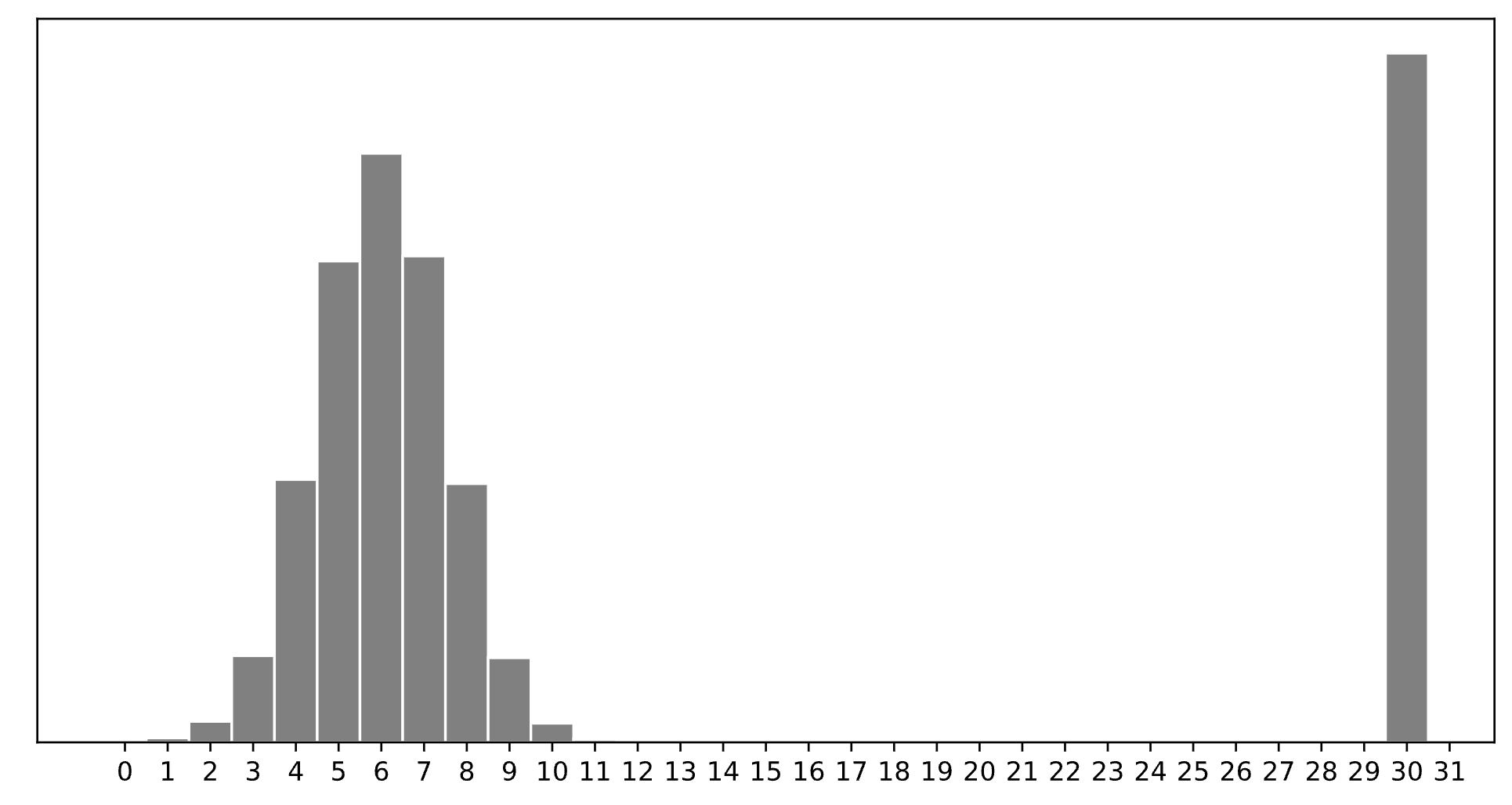
Which of the following is closest to the constant prediction $$w^*$$ that minimizes:

\frac{1}{n} \sum_{i = 1}^n \begin{cases} 0 \quad y_i = w \\\\ 1 \quad y_i \neq w \end{cases}

1 5 6 7 11 15 30

Solution

1 5 6 7 11 15 30

$$30$$ .

The minimizer of average 0-1 loss is the mode.

See: Chapter 1.4: Beyond Absolute and Squared Loss

Which of the following is closest to the constant prediction $$w^*$$ that minimizes:

\frac{1}{n} \sum_{i = 1}^n |y_i - w|

1 5 6 7 11 15 30

Solution

1 5 6 7 11 15 30

$$7$$ .

The minimizer of average absolute loss is the median. The outliers near $$30$$ shift it from $$6$$ to $$7$$ .

Which of the following is closest to the constant prediction $$w^*$$ that minimizes:

\frac{1}{n} \sum_{i = 1}^n (y_i - w)^2

1 5 6 7 11 15 30

Solution

1 5 6 7 11 15 30

$$11$$ .

The minimizer of average squared loss is the mean, pulled upward by the heavy right tail, so it’s above the median ( $$7$$ ) and closest to $$11$$ .

Which of the following is closest to the constant prediction $$w^*$$ that minimizes:

\lim_{p \rightarrow \infty} \frac{1}{n} \sum_{i = 1}^n |y_i - w|^p

Hint: Think about the effect of outliers.

1 5 6 7 11 15 30

Solution

1 5 6 7 11 15 30

$$15$$ .

As $p \to \infty$ , the minimizer is the midrange, halfway between min and max.

Activity 3: Slope of Mean Absolute Error

Consider a dataset of 8 points, $y_1, y_2, \ldots, y_8$ that are in sorted order, i.e. $y_1 < y_2 < \ldots < y_8$ .

Recall that mean absolute error, $R_{\text{abs}}(w)$ , for the constant model $$h(x_i) = w$$ is defined as:

R_{\text{abs}}(w)=\frac{1}{n} \sum_{i=1}^n |y_i - w|

This is a piecewise linear function that changes slope at each data point. The slope of $R_{\text{abs}}(w)$ at any $$w$$ that is not a data point is:

\frac{\text{d}}{\text{d}w} R_{\text{abs}}(w) = \frac{\text{number left of } w - \text{number right of } w}{n}

Suppose that $$y_4=10$$ , $$y_5=14$$ , $$y_6=22$$ , and $R_{\text{abs}}(11)=9$ . What is $R_{\text{abs}}(22)$ ?

Hint: You don’t have all 8 of the $$y$$ -values, so you can’t find $R_\text{abs}(22)$ just by plugging in numbers into the formula for $R_\text{abs}(w)$ . Instead, think about how to use the slope formula.

Solution

$R_{\text{abs}}(22)=11$ .

We can write the points given to us as:

\begin{align*} y_1, y_2, y_3, 10, 14, 22, y_7, y_8 \end{align*}

Since there are an even number of data points ( $$n=8$$ ), the minimizer of absolute error is not a single point but the entire interval between the two middle points. Here, the middle two are $$10$$ and $$14$$ , so every $w \in [10,14]$ minimizes $R_{\text{abs}}(w)$ . This explains why the error is flat inside that interval: the number of points on the left equals the number on the right, so shifting $$w$$ around does not change the error. As a result, $R_{\text{abs}}(11)=9$ and $R_{\text{abs}}(14)=9$ .

Once we move beyond $$14$$ , the balance breaks. There are now five points to the left and only three to the right, so the slope of $R_{\text{abs}}(w)$ becomes positive. The slope formula tells us:

\frac{d}{dw}R_{\text{abs}}(w) = \frac{\text{number left of } w - \text{number right of } w}{n}

so for any $w \in (14,22)$ we have

\frac{d}{dw}R_{\text{abs}}(w) = \frac{5-3}{8} = \tfrac{1}{4}.

This means that for every one unit we move to the right of $$w=14$$ , the error increases by $\tfrac{1}{4}$ . Moving from $$w=14$$ to $$w=22$$ is a distance of $$22-14=8$$ units, so the error increases by

8 \cdot \tfrac{1}{4} = 2.

Adding this to the baseline error of $R_{\text{abs}}(14)=9$ , we get:

\begin{align*} R_{\text{abs}}(22) &= R_{\text{abs}}(14) + (22-14)\cdot \tfrac{1}{4} \\\\ &= 9 + 2 = 11. \end{align*}

Activity 4: Programming

Complete the tasks in the lab02.ipynb notebook.

There are two ways to access the supplemental Jupyter Notebook:

Option 1 (preferred): Set up a Jupyter Notebook environment locally, use git to clone our course repository, and open labs/lab02/lab02.ipynb. For instructions on how to do this, see the Environment Setup page of the course website.
Option 2: Click here to open lab02.ipynb on DataHub. Before doing so, read the instructions on the Environment Setup page on how to use the DataHub.

Once you’re done, include a screenshot of your completed Activity 4 implementation in your PDF submission of Lab 2 to Gradescope, making sure to include proof that the (local) autograder passed.

Activity 5: Reverse Regression

Suppose we have a dataset of $$n$$ houses that were recently sold in the Ann Arbor area. For each house, we have its square footage and most recent sale price. The correlation between square footage and price is $$r$$ .

First, we minimize mean squared error to fit a simple linear model that uses square footage to predict price. The resulting regression line has an intercept of $$w_0^*$$ and slope of $$w_1^*$$ .

\text{predicted price}_i=w_0^*+w_1^* \cdot \text{square footage}_i

We’re now interested in minimizing mean squared error to fit a simple linear model that uses price to predict square footage — that is, we’re “reversing” the $$x$$ and $$y$$ variables. Suppose this new regression line has an intercept of $\beta_0^*$ and slope of $\beta_1^*$ .

Find $\beta_1^*$ . Give your answer in terms of one or more of $$n$$ , $$r$$ , $$w_0^*$$ , and $$w_1^*$$ .

Solution

Let $$x$$ represent square footage and $$y$$ represent price.

We know that $w_1^*=r\frac{\sigma_y}{\sigma_x}$ . But what about $\beta_1^*$ ?

When we take a rule that predicts price from square footage and transform it into a rule that predicts square footage from price, the roles of $$x$$ and $$y$$ have swapped; suddenly, square footage is no longer our independent variable, but our dependent variable, and vice versa for price. This means that the altered dataset we work with when using our new prediction rule has $\sigma_x$ standard deviation for its dependent variable (square footage), and $\sigma_y$ for its independent variable (price). So, we can write the formula for $\beta_1^*$ as follows:

\beta_1^*=r\frac{\sigma_x}{\sigma_y}

In essence, swapping the independent and dependent variables of a dataset changes the slope of the regression line from $r\frac{\sigma_y}{\sigma_x}$ to $r\frac{\sigma_x}{\sigma_y}$ . Now, let’s simplify to get rid of the $\sigma_x$ and $\sigma_y$ :

\begin{align*} \beta_1^*&=r\frac{\sigma_x}{\sigma_y} \\\\w_1^* \cdot \beta_1^*&=w_1^* \cdot r\frac{\sigma_x}{\sigma_y} \\\\w_1^* \cdot \beta_1^*&=r\frac{\sigma_y}{\sigma_x} \cdot r\frac{\sigma_x}{\sigma_y} \\\\w_1^* \cdot \beta_1^*&=r\cdot r \\\\\beta_1^*&=\frac{r^2}{w_1^*} \end{align*}

Activity 6: Transformed Data

Suppose we’re given a dataset of $$n$$ points, $(x_1, y_1), (x_2, y_2), \dots, (x_n, y_n)$ , where $\bar{x}$ is the mean of $x_1, x_2, \dots, x_n$ and $\bar{y}$ is the mean of $y_1, y_2, \dots, y_n$ .

Using this dataset, we create a transformed dataset of $$n$$ points, $(x_1', y_1'), (x_2', y_2'), \dots, (x_n', y_n')$ , where:

x_i' = 4x_i - 3 \qquad y_i' = y_i + 24

So the transformed dataset is of the form

(4x_1-3, y_1+24), (4x_2-3, y_2+24), \dots, (4x_n-3, y_n+24)

We decide to fit a simple linear model $$h(x_i') = w_0 + w_1 x_i'$$ on the transformed dataset using squared loss. We find that $$w_0^* = 7$$ and $$w_1^* = 2$$ , so $$h^*(x_i') = 7 + 2x_i'$$ .

Suppose we were to fit a simple linear model through the original dataset, $(x_1, y_1), (x_2, y_2), \dots, (x_n, y_n)$ , again using squared loss. What would the optimal slope on the original dataset be?

Solution

Relative to the dataset with $$x'$$ , the dataset with $$x$$ is compressed by a factor of 4, so the slope increases by a factor of 4: $2 \cdot 4 = 8$ .

Concretely, this can be shown by looking at the formula for the new slope:

\begin{align*} 2 &= r\frac{\sigma_{y'}}{\sigma_{x'}} \\\\ 2 &= r\frac{\sigma_y}{4\sigma_x} \\\\ 8 &= r\frac{\sigma_y}{\sigma_x} \end{align*}

so the original slope is $$8$$ .

Recall, the model $$h^*(x_i') = w_0 + w_1 x_i'$$ was fit on the transformed dataset, $(x_1', y_1'), (x_2', y_2'), \dots, (x_n', y_n')$ . $$h^*(x_i')$$ happens to pass through the point $(\bar{x}, \bar{y})$ . What is the value of $\bar{x}$ ? Give your answer as an integer with no variables. Hint: What else does $$h^*(x_i')$$ pass through?

Solution

$$h^*(x_i')$$ is guaranteed to pass through $(\bar{x}', \bar{y}')$ , where $\bar{x}'$ is the mean of the $$x'$$ values and $\bar{y}'$ is the mean of the $$y'$$ values.

Let’s see what that looks like as an equation:

\begin{align*} w_0^* + w_1^*\bar{x}' &= h^*(\bar{x}') \\\\ 7 + 2\bar{x}' &= h^*(\bar{x}') \\\\ 7 + 2\bar{x}' &= \bar{y}' \end{align*}

Now write $\bar{x}'$ and $\bar{y}'$ in terms of $\bar{x}$ and $\bar{y}$ :

\bar{x}' = 4\bar{x} - 3 \qquad \bar{y}' = \bar{y} + 24

Substitute these into the equation above:

7 + 2(4\bar{x} - 3) = \bar{y} + 24

The problem also tells us that $$h^*(x_i')$$ passes through $(\bar{x}, \bar{y})$ , so

2\bar{x} + 7 = \bar{y}

Now subtract:

\begin{align*} 7 + 2(4\bar{x} - 3) - (2\bar{x} + 7) &= \bar{y} + 24 - \bar{y} \\\\ 7 + 8\bar{x} - 6 - 2\bar{x} - 7 &= 24 \\\\ 6\bar{x} &= 30 \\\\ \bar{x} &= 5 \end{align*}

The following are extra practice. Don’t feel pressured to answer all of these problems in lab, but make sure to attempt them at some point.

Activity 7: Relative Squared Loss, Continued

Recall the formula for relative squared loss from Activity 1:

L_{\text{rsq}}(y_i, h(x_i)) = \frac{(y_i - h(x_i))^2}{y_i}

Let $$C(y_1, y_2, \dots, y_n)$$ be your minimizer $$w^*$$ from Activity 1. That is, for a particular dataset $$y_1, y_2, \dots, y_n$$ , $$C(y_1, y_2, \dots, y_n)$$ is the value of $$w$$ that minimizes empirical risk for relative squared loss on that dataset.

What is the value of $\displaystyle\lim_{y_4 \rightarrow \infty} C(1, 3, 5, y_4)$ in terms of $$C(1, 3, 5)$$ ? Your answer should involve the function $$C$$ and/or one or more constants.

Hint: To notice the pattern, evaluate $$C(1, 3, 5, 100)$$ , $$C(1, 3, 5, 10000)$$ , and $$C(1, 3, 5, 1000000)$$ .

Solution

\begin{align*} \lim_{y_4 \rightarrow \infty} C(1, 3, 5, y_4) &= \lim_{y_4 \rightarrow \infty} \frac{4}{\frac{1}{1} + \frac{1}{3} + \frac{1}{5} + \frac{1}{y_4}} \\\\ &= \frac{4}{\frac{1}{1} + \frac{1}{3} + \frac{1}{5} + 0} \\\\ &= \frac{4}{3} \cdot \frac{3}{\frac{1}{1} + \frac{1}{3} + \frac{1}{5}} \\\\ &= \frac{4}{3} \cdot C(1, 3, 5) \end{align*}

What is the value of $\displaystyle\lim_{y_4 \rightarrow 0} C(1, 3, 5, y_4)$ ? Again, your answer should involve the function $$C$$ and/or one or more constants.

Solution

\begin{align*} \lim_{y_4 \rightarrow 0} C(1, 3, 5, y_4) &= \lim_{y_4 \rightarrow 0} \frac{4}{\frac{1}{1} + \frac{1}{3} + \frac{1}{5} + \frac{1}{y_4}} \\\\ &= \frac{4}{\frac{1}{1} + \frac{1}{3} + \frac{1}{5} + \infty} \\\\ &= \frac{4}{\infty} = 0 \end{align*}

Based on the results of the previous two parts, when is the prediction $$C(y_1, y_2, \dots, y_n)$$ robust to outliers? When is it not robust to outliers?

Solution

$$C(y_1, y_2, \dots, y_n)$$ is great at ignoring large outliers. No matter how large you make any particular value, $$C(y_1, y_2, \dots, y_n)$$ is upper-bounded by $\frac{n}{n-1}$ multiplied by the value of $$C$$ applied to all data points excluding the large outlier. This is as opposed to the regular “arithmetic mean”, where if you make a single data point arbitrarily large, the mean also becomes arbitrarily large (i.e. if $y_n \rightarrow \infty$ , then $\text{Mean}(y_1, y_2, …, y_n) \rightarrow \infty$ too).

However, $$C(y_1, y_2, \dots, y_n)$$ is not robust to small outliers. As a particular data point approaches 0, the value of $$C(y_1, y_2, \dots, y_n)$$ also approaches 0 no matter how large the other data points are.

Activity 8: The Meaning of Mean Squared Error

Suppose we’d like to predict the number of minutes a delivery will take, $$y$$ , as a function of distance, $$x$$ . To do so, we look to our dataset of $$n$$ deliveries, $(x_1, y_1), (x_2,y_2), \dots, (x_n,y_n)$ , and fit two simple linear models:

$$F(x_i)=a_0+a_1x_i$$ , where:

a_1=r\frac{\sigma_y}{\sigma_x}, \qquad a_0=\bar y - a_1 \bar x

Here, $$r$$ is the correlation coefficient between $$x$$ and $$y$$ , $\bar x$ and $\bar y$ are their respective means, and $\sigma_x$ and $\sigma_y$ are their respective standard deviations.

$$G(x_i)=b_0+b_1x_i$$ , where $$b_0$$ and $$b_1$$ are chosen such that $$G(x_i)=b_0+b_1x_i$$ minimizes mean absolute error on the dataset. Assume that no other line minimizes mean absolute error on the dataset, i.e. that the values of $$b_0$$ and $$b_1$$ are unique.

Fill in the $\boxed{???}$ :

\displaystyle \sum_{i=1}^{n}(y_i-F(x_i))^2 \quad \boxed{???} \quad \sum_{i=1}^{n}(y_i-G(x_i))^2

$>$ $\geq$ $=$ $\leq$ $<$ Impossible to tell

Solution

$>$ $\geq$ $=$ $\leq$ $<$ Impossible to tell

The quantity on the left hand side is the total squared error of model $$F$$ . By definition, $$F$$ , is the line that minimizes MSE over all possible linear models.

The quantity on the right hand side is the total squared error of model $$G$$ . However, $$G$$ is optimized for mean absolute error, not MSE.

The question tells us that $$F$$ and $$G$$ are different, so $\displaystyle \sum_{i=1}^{n}(y_i-F(x_i))^2 < \sum_{i=1}^{n}(y_i-G(x_i))^2$ must be true.

Fill in the $\boxed{???}$ :

\displaystyle \left(\sum_{i=1}^{n}|y_i-F(x_i)|\right)^2 \quad \boxed{???} \quad \left(\sum_{i=1}^{n}|y_i-G(x_i)|\right)^2

$>$ $\geq$ $=$ $\leq$ $<$ Impossible to tell

Solution

$>$ $\geq$ $=$ $\leq$ $<$ Impossible to tell

The quantity on the left hand side is the squared total absolute error of model $$F$$ .

The quantity on the right hand side is the squared total absolute error of model $$G$$ . By definition, $$G$$ , is the line that minimizes MAE over all possible linear models.

The total absolute error of $$G$$ must be less than the total absolute error of $$F$$ , and squaring them doesn’t change that relationship because both totals are guaranteed to be positive numbers (sums of absolute values).

Finally, $$F$$ and $$G$$ are different, so $\displaystyle \left(\sum_{i=1}^{n}|y_i-F(x_i)|\right)^2 > \left(\sum_{i=1}^{n}|y_i-G(x_i)|\right)^2$

Below, we’ve drawn the lines for both $$F$$ and $$G$$ along with a scatter plot for the original $$n$$ deliveries:

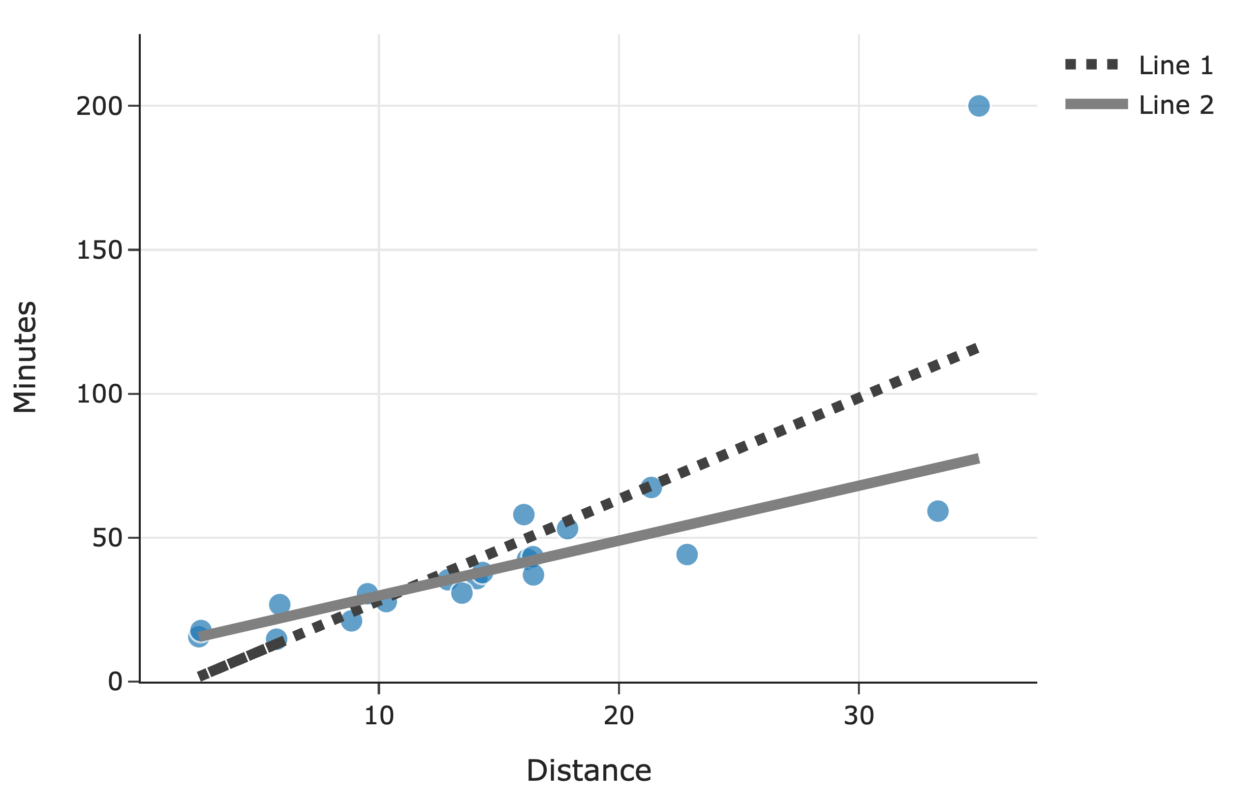
Which line corresponds to $$F$$ ?

Line 1 Line 2

Solution

Line 1 Line 2

Line 1

The key idea is that models trained with squared loss (MSE) are more sensitive to outliers than models trained with absolute loss (MAE).

Since Line 1 appears to be “pulled up” more strongly by an outlier, it suggests that this line was influenced more heavily by extreme values. This behavior aligns with how MSE-based regression works: outliers have a greater impact on the overall loss because squaring the errors makes large deviations even more significant.

In contrast, MAE-based regression (Line 2) is less sensitive to outliers because absolute differences do not grow as quickly.

Therefore, Line 1 corresponds to $$F$$ , the MSE-minimizing line.

Activity 9: What Do You Mean?

Suppose we want to fit a simple linear model (using squared loss) that predicts the number of ingredients in a product given its price. We’re given that:

The average cost of a product in our dataset is $40, i.e. $\bar x=40$
The average number of ingredients in a product in our dataset is 15, i.e. $\bar y =15$

The intercept and slope of the regression line are $$w_0^*=11$$ and $w_1^*=\frac{1}{10}$ , respectively.

Suppose Victors’ Veil (a skincare product) costs $40 and has 11 ingredients. What is the squared loss of our model’s predicted number of ingredients for Victors’ Veil?

Solution

Using the equation of the regression model we have seen in class:

$$ h(x_i)=w_0^*+w_1^*x_i $$

Plugging in $$w_0^*=11$$ , $w_1^*=\frac{1}{10}$ , and $$x=40$$ gives us:

h(x_i)=11+\frac{1}{10}\cdot 40 = 15

The squared loss is $$L=(y_i-h(x_i))^2$$ , substituting $$y=11$$ (actual) and $$h(x_i)=15$$ (predicted) gives us:

$$ L=(11-15)^2=16 $$

Is it possible to answer part a) above just by knowing $\bar x$ and $\bar y$ , i.e. without knowing the values of $$w_0^*$$ and $$w_1^*$$ ? Once you select an answer, explain it to your peers.

Yes, it's possible No, it's not possible

Solution

Yes, it's possible No, it's not possible

Yes, the values of $$w_0^*$$ and $$w_1^*$$ don’t impact the answer to part a).

The simple linear model minimizing mean squared error will always go through the point $(\bar x, \bar y)$ . We’re given $\bar x=40$ and $\bar y=15$ , meaning that for a product that costs $40 we will predict that it has 15 ingredients, no matter what the slope and intercept end up being.

Activity 10: A Refresher

Consider a dataset of $y_1, y_2, \dots, y_n$ , all of which are positive. We want to fit a constant model, $$h(x_i)=w$$ , to the data.

Let $$w_p^*$$ be the optimal constant prediction that minimizes average degree- $$p$$ loss, $$R_p(w)$$ , defined below:

R_p(w)= \displaystyle \frac{1}{n} \sum_{i=1}^{n}|y_i-w|^p

For example, $$w_2^*$$ is the optimal constant prediction that minimizes $R_2(w)= \displaystyle \frac{1}{n} \sum_{i=1}^{n}|y_i-w|^2$

In each of the parts below, determine the value of the quantity provided. By “the data”, we are referring to $y_1, y_2, \dots, y_n$ . The answer choices are as follows; select one item in each row.

A: The standard deviation of the data
B: The variance of the data
C: The mean of the data
D: The median of the data
E: The midrange of the data, $\frac{y_\text{min} + y_\text{max}}{2}$
F: The mode of the data
G: None of these

		A	B	C	D	E	F	G
$$i$$	$$h_0^*$$
$$ii$$	$$h_1^*$$
$$iii$$	$$R_1(h_1^*)$$
$$iv$$	$$h_2^*$$
$$v$$	$$R_2(h_2^*)$$

Solution

$$h_0^*$$ is none of the these. The original intention was to have $$R_0$$ be 0-1 loss, in which case $$h_0^*$$ would be the mode.
$$h_1^*$$ is the median of the data, since $R_1(w)= \displaystyle \frac{1}{n} \sum_{i=1}^{n}|y_i-w|$
$$R_1(h_1^*)$$ is the minimum mean absolute error, which is none of these.
$$h_2^*$$ is the mean of the data, since $R_2(w)= \displaystyle \frac{1}{n} \sum_{i=1}^{n}|y_i-w|^2$ is equivalent to mean squared error.
$$R_2(h_2^*)$$ is the variance of the data, or the minimum mean absolute error, shown below:

\begin{align*} R_2(h_2^*)&=\displaystyle \frac{1}{n} \sum_{i=1}^{n}|y_i-h_2^*|^2 \&=\displaystyle \frac{1}{n} \sum_{i=1}^{n}|y_i-\bar y|^2 \&=\displaystyle \frac{1}{n} \sum_{i=1}^{n}(y_i-\bar y)^2 = \sigma_y^2 \end{align*}

Now, suppose we want to find the optimal constant prediction, $h_\text{U}^*$ , using the “Ulta” loss function, defined below:

L_\text{U}(y_i, w) = y_i(y_i-w)^2

To find $h_\text{U}^*$ , we minimize $R_\text{U}(w)$ , the average Ulta loss. How does $h_\text{U}^*$ compare to the mean of the data, $$M$$ ?

$h_\text{U}^* > M$ $h_\text{U}^* \geq M$ $h_\text{U}^* = M$ $h_\text{U}^* \leq M$ $h_\text{U}^* < M$

Solution

$h_\text{U}^* > M$ $h_\text{U}^* \geq M$ $h_\text{U}^* = M$ $h_\text{U}^* \leq M$ $h_\text{U}^* < M$

Minimizing the average Ulta loss means minimizing the empirical risk:

R_\text{U}(w)=\displaystyle \frac{1}{n} \sum_{i=1}^{n}y_i(y_i-w)^2

This resembles minimizing mean squared error, except each $$y_i$$ is given a weight of $$y_i$$ . All the $$y_i$$ values are positive, so larger $$y_i$$ values contribute more to the loss. To reduce their impact of these large $$y_i$$ values, the minimizer gets pulled higher, causing it to be greater than the mean.

Finally, to find the optimal constant prediction, we will instead minimize regularized average Ulta loss, $R_\lambda(w)$ , defined below:

\displaystyle R_\lambda(w) = \left(\frac{1}{n} \sum_{i=1}^{n} y_i(y_i-w)^2\right)+\lambda w^2

Here, assume $\lambda > 0$ is some positive constant. (We will cover regularization in more detail later in the term.)

Find $$w^*$$ , the constant prediction that minimizes $R_\lambda(w)$ . Give your answer as an expression in terms of the $$y_i$$ ’s, $$n$$ , and/or $\lambda$ .

Solution

To minimize the regularized average Ulta loss, we solve for $$w$$ by setting $\displaystyle \frac{\partial R}{\partial w}=0$ and solving for $$w$$ .

Step 1: Compute the derivative and set to 0.

\begin{align*} \displaystyle \frac{\partial R}{\partial w}R_\lambda(w) &= \frac{\partial}{\partial w}\left[\left(\frac{1}{n} \sum_{i=1}^{n} y_i(y_i-w)^2\right)+\lambda w^2\right] \&=-2\left(\frac{1}{n} \sum_{i=1}^{n} y_i(y_i-w)\right)+2\lambda w = 0 \end{align*}

Step 2: Expand and simplify.

\begin{align*} -2\left(\frac{1}{n} \sum_{i=1}^{n} y_i(y_i-w)\right)+2\lambda w &= 0 \\\\\frac{1}{n} \sum_{i=1}^{n} y_i(y_i-w)-\lambda w &= 0 \\\\\frac{1}{n} \sum_{i=1}^{n} y_i^2 - \frac{1}{n} \sum_{i=1}^{n} y_iw-\lambda w &= 0 \\\\\frac{1}{n} \sum_{i=1}^{n} y_i^2 &= \frac{1}{n} \sum_{i=1}^{n} y_iw+\lambda w \end{align*}

Step 3: Solve for $$w$$ .

\begin{align*} \frac{1}{n} \sum_{i=1}^{n} y_i^2 &= \frac{1}{n} \sum_{i=1}^{n} y_iw+\lambda w \\\\\frac{1}{n} \sum_{i=1}^{n} y_i^2 &= w\left(\frac{1}{n} \sum_{i=1}^{n} y_i+\lambda\right) \\\\\frac{\frac{1}{n} \sum_{i=1}^{n} y_i^2}{\frac{1}{n} \sum_{i=1}^{n} y_i+\lambda} &= w \end{align*}

Step 4: Multiply by $\frac{n}{n}$

w^* = \frac{\sum_{i=1}^{n} y_i^2}{\sum_{i=1}^{n} y_i+\lambda}

		A	B	C	D	E	F	G
$\(i\)$	$\(h_0^*\)$
$\(ii\)$	$\(h_1^*\)$
$\(iii\)$	$\(R_1(h_1^*)\)$
$\(iv\)$	$\(h_2^*\)$
$\(v\)$	$\(R_2(h_2^*)\)$