Find \(f\left(\begin{bmatrix} 2 \\ 1 \\ 2 \end{bmatrix}\right)\). After that, find the matrix \(A\) corresponding to \(f\), i.e. where \(f(\vec x) = A \vec x\).
Lab 7: Inverses and Projections
due for completion at 11:59PM Ann Arbor Time on Monday, June 1st, 2026
Each lab worksheet will contain several activities, some of which will involve writing code and others that will involve writing math on paper. To receive credit for a lab, you must complete as many of the activities as you can in 2 hours and submit a PDF of your work to Gradescope. We will provide specific instructions on how to submit programming activities (e.g. submitting the notebook or including a screenshot of some output).
Activities
- Activity 1: PrairieLearn Practice Problems
- Activity 2: Linear Transformations
- Activity 3: Projecting onto the Column Space
Recap: Inverses (Chapter 6.2) and Linear Transformations (Chapter 6.1)
(We provide a recap of projections and the normal equation in Activity 3.)
An \(n \times n\) square matrix \(A\) is invertible if and only if \(\text{rank}(A) = n\), which also means that \(A\)’s columns are linearly independent (along with several other equivalent conditions).
If \(A\) is invertible, then its inverse \(A^{-1}\) is the unique \(n \times n\) matrix such that \(AA^{-1}=I=A^{-1}A\).
The determinant of a square matrix \(A\) is the volume of the \(n\)-dimensional cube with side length 1 after it is transformed by \(A\).
If \(\text{det}(A) = 0\), then \(A\) is not invertible.
If \(A = \begin{bmatrix} a & b \\ c & d \end{bmatrix}\), then \(\text{det}(A) = ad - bc\) and \(A^{-1} = \frac{1}{ad - bc} \begin{bmatrix} d & -b \\ -c & a \end{bmatrix}\).
The determinant satisfies several properties, including that \(\text{det}(AB) = \text{det}(A) \text{det}(B)\) and \(\text{det}(A^T) = \text{det}(A)\).
A linear transformation is a function \(\mathbb{R}^d \to \mathbb{R}^n\) such that
$$ f(\vec x + \vec y) = f(\vec x) + f(\vec y), \qquad f(c \vec x) = c f(\vec x) $$
Every linear transformation has a corresponding \(n \times d\) matrix \(A\) where \(f(\vec x) = A \vec x\).
If \(A\) is square, then \(f(\vec x) = A \vec x\) is a function from \(\mathbb{R}^n\) to \(\mathbb{R}^n\), and \(A\) is invertible if and only if the function \(f\) is invertible.
Activity 1: PrairieLearn Practice Problems
We’re testing out a new website for practicing linear algebra problems: PrairieLearn.
Click this link to access the relevant problems for this activity. It consists of 6 problems, each worth 1 point. The numbers in the problems are randomized; everyone will receive slightly different problems.
To get credit for Activity 1, you must eventually correctly answer all 6 problems, earning a score of 6/6. If you answer a problem incorrectly, click “New Variant” to generate a new version and then try again. There is no penalty for answering a problem incorrectly, as long as you eventually get it correct.
To be clear, you don’t need to include anything in your PDF for Activity 1; we will manually verify that you’ve finished all 6 problems.
If you have trouble accessing PrairieLearn, message Suraj on Slack.
Activity 2: Linear Transformations
Suppose \(f: \mathbb{R}^3 \to \mathbb{R}^3\) is a linear transformation represented by the matrix \(A\).
Furthermore, suppose that \(f\left(\begin{bmatrix} 1 \\ 0 \\ 0 \end{bmatrix}\right) = \begin{bmatrix} 0 \\ 3 \\ 4 \end{bmatrix}\), \(f\left(\begin{bmatrix} 0 \\ 10 \\ 0 \end{bmatrix}\right) = \begin{bmatrix} 0 \\ 4 \\ -3 \end{bmatrix}\), and \(f\left(\begin{bmatrix} 0 \\ 0 \\ 1 \end{bmatrix}\right) = \begin{bmatrix} 1 \\ 0 \\ 0 \end{bmatrix}\).
a)
b)
Find a diagonal matrix \(D\) and an orthogonal matrix \(Q\) such that \(A = QD\). (Not every matrix can be written in this form, but this particular \(A\) can.) Then, describe in English how \(f\) transforms a vector \(\vec x\).
c)
Using your \(A = QD\) decomposition from part b), find \(A^{-1}\).
Hint: Recall that for orthogonal matrices, \(QQ^T = Q^TQ = I\). And, for any invertible matrices \(A\) and \(B\), \((AB)^{-1} = B^{-1}A^{-1}\).
d)
Given the English definition of \(f\) from part b) alone, find \(\text{det}(A)\). (You can verify your work using the formula in Chapter 6.1.)
Activity 3: Projecting onto the Column Space
Note: We’ve recorded a YouTube playlist walking through the activities in this lab.
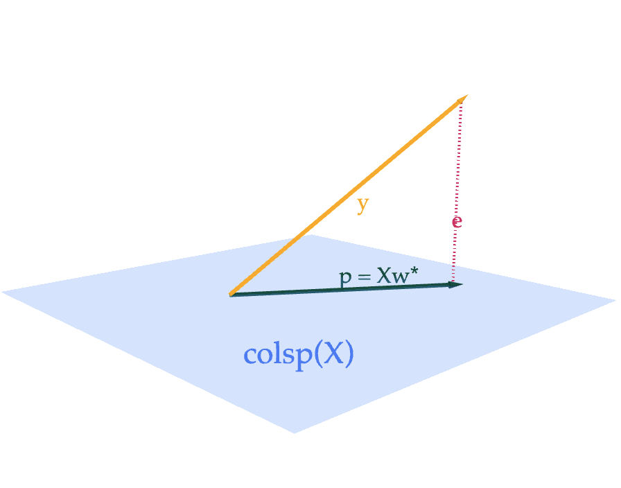
Suppose \(X\) is an \(n \times d\) matrix with columns \(\vec x^{(1)}, \vec x^{(2)}, \ldots, \vec x^{(d)}\) and \(\vec y \in \mathbb{R}^n\). Then, the projection of \(\vec y\) onto \(\text{colsp}(X)\) is the vector
$$ \vec p = X\vec w^* = w_1^* \vec x^{(1)} + w_2^* \vec x^{(2)} + \cdots + w_d^* \vec x^{(d)} $$
where \(\vec w^* \in \mathbb{R}^d\) is chosen to satisfy the normal equation,
$$ X^TX \vec w = X^T \vec y $$
If \(X\)’s columns are linearly independent, \(\vec w^*\) is the unique vector
$$ \vec w^* = (X^TX)^{-1}X^T \vec y $$
Of all vectors in \(\text{colsp}(X)\), \(X \vec w^*\) is the one that is closest to \(\vec y\), meaning it minimizes
$$ \lVert \vec y - X \vec w \rVert^2 $$
As we will see in Tuesday’s lecture, \(\vec w^*\) contains the optimal model parameters for linear regression, when we fill our \(X\) (carefully) with our input variables and \(\vec y\) with our output variables.
a)
Let \(X = \begin{bmatrix} 2 & 1 \\ 0 & -3 \\ 0 & 0 \end{bmatrix}\) and \(\vec y = \begin{bmatrix} 2 \\ 3 \\ 4 \end{bmatrix}\). Find \(\vec w^*\), \(\vec p\), and \(\vec e = \vec y - \vec p\), and verify that \(\vec e\) is orthogonal to \(\text{colsp}(X)\) by showing that it is orthogonal to each of \(X\)’s columns.
b)
Find scalars \(a\) and \(b\) such that \(a \begin{bmatrix} 2 \\ 0 \\ 0 \end{bmatrix} + b \begin{bmatrix} 1 \\ -3 \\ 0 \end{bmatrix}\) is as close as possible to \(\begin{bmatrix} 1 \\ 9 \\ 2 \end{bmatrix}\). Hint: You can reuse most of your work from part a).
c)
Now, suppose \(X = \begin{bmatrix} 1 & 1 \\ 1 & -1 \\ 1 & 0 \end{bmatrix}\) and \(\vec y = \begin{bmatrix} 2 \\ 3 \\ 4 \end{bmatrix}\). We’ve already computed \(\vec w^*\), \(\vec p\), and \(\vec e\) here:
$$ \vec w^* = \begin{bmatrix} 3 \\\\ -\frac{1}{2} \end{bmatrix}, \quad \vec p = \begin{bmatrix} 5/2 \\\\ 7/2 \\\\ 3 \end{bmatrix}, \quad \vec e = \vec y - \vec p = \begin{bmatrix} -1/2 \\\\ -1/2 \\\\ 1 \end{bmatrix} $$
Notice that the components of this \(\vec e\) add up to 0, but this doesn’t happen with your \(\vec e\) from part a). Why? Hint: The answer is not that \(\vec y\) is in \(\text{colsp}(X)\) — it isn’t in part a) and it isn’t here either. Rather, it has something to do with the difference between the two \(X\)’s. This is a hugely important result, and one that will 100% appear on Midterm 2.
Taking another look at the formula \(\vec p = X \vec w^*\), we see that it’s equivalent to
$$ \vec p = X \vec w^* = X (X^TX)^{-1}X^T\vec y = P\vec y $$
where \(P = X (X^TX)^{-1}X^T\) is called the projection matrix, discussed in Chapter 6.4. Multiplying \(P \vec y\) is equivalent to projecting \(\vec y\) onto \(\text{colsp}(X)\).
d)
Recall that \(X\) is an \(n \times d\) matrix (meaning it’s not necessarily square), which makes \(P = X (X^TX)^{-1}X^T\) an \(n \times n\) matrix.
Fill in the blanks: \(X^TX\) is invertible if and only if \(X\)’s columns are ____.
e)
In this part only, suppose \(X\) is an \(n \times 1\) matrix, i.e. it is a vector. Then,
What is the value of \(\vec w^*\), and how does it relate to what we learned in Chapter 3.4? (What type of object is \((X^TX)^{-1}\) when \(X\) is a vector?)
What is the value of the matrix \(P\), and how does it relate to what we learned in Homework 6, Problem 5?
$$ P = X (X^TX)^{-1}X^T $$
f)
Show that \(P\) is both symmetric (meaning that \(P^T = P\)) and idempotent (meaning that \(P^2 = P\)). Then, explain in English how \(P\)’s idempotence relates to the linear transformation of projecting \(\vec y\) onto \(\text{colsp}(X)\).
g)
In the rare case that \(X\) is an \(n \times n\) square matrix, and \(\text{rank}(X) = n\), what is \(P\)? What does this say about the relationship between \(\vec y\), \(\vec p\), and \(\text{colsp}(X)\)? Hint: Use the fact that \((AB)^{-1} = B^{-1}A^{-1}\).