Lab 11: Adjacency Matrices and Diagonalization

due for completion at 11:59PM Ann Arbor Time on Wednesday, June 17th, 2026

Each lab worksheet will contain several activities, some of which will involve writing code and others that will involve writing math on paper. To receive credit for a lab, you must complete as many of the activities as you can in 2 hours and submit a PDF of your work to Gradescope. We will provide specific instructions on how to submit programming activities (e.g. submitting the notebook or including a screenshot of some output).

Feel free to work with others in the course, but you must submit individually.


Activities


Recap: Diagonalization (Chapter 9.4)

  • Since \(A\) has two linearly independent eigenvectors, it is diagonalizable, meaning we can write
$$ A = V \Lambda V^{-1} = \underbrace{\begin{bmatrix} 2 & 3 \\\\ -6 & 1 \end{bmatrix}}_{V} \underbrace{\begin{bmatrix} -3 & 0 \\\\ 0 & 7 \end{bmatrix}}_{\Lambda} \underbrace{\begin{bmatrix} 0.05 & -0.15 \\\\ 0.3 & 0.1 \end{bmatrix}}_{V^{-1}} $$

where \(V\) is an invertible matrix whose columns are the eigenvectors of \(A\) and \(\Lambda\) is a diagonal matrix with the eigenvalues of \(A\) on the diagonal.

  • The algebraic multiplicity of an eigenvalue, \(\text{AM}(\lambda_i)\), is the number of times it appears as a root of the characteristic polynomial.
$$ p(\lambda) = (\lambda - \lambda_1)^{\text{AM}(\lambda_1)} (\lambda - \lambda_2)^{\text{AM}(\lambda_2)} \cdots (\lambda - \lambda_k)^{\text{AM}(\lambda_k)} $$
  • The geometric multiplicity of an eigenvalue, \(\text{GM}(\lambda_i)\), is the dimension of the eigenspace corresponding to \(\lambda_i\).
$$ \text{GM}(\lambda_i) = \text{dim}(\text{nullsp}(A - \lambda_i I)) = \text{number of linearly independent eigenvectors corresponding to } \lambda_i $$
  • For any \(\lambda_i\), \(1 \leq \text{GM}(\lambda_i) \leq \text{AM}(\lambda_i)\).

  • \(A\) is diagonalizable if and only if \(\text{AM}(\lambda_i) = \text{GM}(\lambda_i)\) for all eigenvalues \(\lambda_i\). This ensures that \(A\)’s eigenvectors form a basis of \(\mathbb{R}^n\).

  • \(A = \begin{bmatrix} 3 & -1 \\ 1 & 1 \end{bmatrix}\) has characteristic polynomial \(p(\lambda) = (2 - \lambda)^2\). The eigenvalue \(\lambda = 2\) has algebraic multiplicity 2, but the corresponding eigenspace is only 1-dimensional:

$$ \text{nullsp}(A - 2I) = \text{nullsp}\left(\begin{bmatrix} 1 & -1 \\\\ 1 & -1 \end{bmatrix}\right) = \text{span}\left(\begin{bmatrix} 1 \\\\ 1 \end{bmatrix}\right) $$

so, \(\lambda = 2\) has geometric multiplicity 1. Since \(\text{AM}(2) \neq \text{GM}(2)\), \(A\) is not diagonalizable.

  • \(A = \begin{bmatrix} 1 & 0 & 0 \\ -1 & 2 & 1 \\ -1 & 1 & 2 \end{bmatrix}\) has characteristic polynomial \(p(\lambda) = (1 - \lambda)^2(3 - \lambda)\), so \(\lambda_1 = 1\) has \(\text{AM}(\lambda_1) = 2\) and \(\lambda_2 = 3\) has \(\text{AM}(\lambda_2) = 1\). The eigenspace for \(\lambda_1 = 1\) is 2-dimensional,
$$ \text{nullsp}(A - 1 I) = \text{nullsp}\left(\begin{bmatrix} 0 & 0 & 0 \\\\ -1 & 1 & 1 \\\\ -1 & 1 & 1 \end{bmatrix}\right) = \text{span}\left(\begin{bmatrix} 1 \\\\ 1 \\\\ 0 \end{bmatrix}, \begin{bmatrix} 1 \\\\ 0 \\\\ 1 \end{bmatrix}\right) $$

so \(\text{GM}(\lambda_1) = 2\). Since \(\text{AM}(\lambda_i) = \text{GM}(\lambda_i)\) for all eigenvalues \(\lambda_i\), \(A\) is diagonalizable.

$$ A = V \Lambda V^{-1} = \underbrace{\begin{bmatrix} 1 & 1 & 0 \\\\ 1 & 0 & 1 \\\\ 0 & 1 & 1 \end{bmatrix}}_{V} \underbrace{\begin{bmatrix} 1 & 0 & 0 \\\\ 0 & 1 & 0 \\\\ 0 & 0 & 3 \end{bmatrix}}_{\Lambda} \underbrace{\begin{bmatrix} 0.5 & 0.5 & -0.5 \\\\ 0.5 & -0.5 & 0.5 \\\\ -0.5 & 0.5 & 0.5 \end{bmatrix}}_{V^{-1}} $$
  • Diagonalizability is not the same as invertibility!

Activity 1: Rapid Fire

The goal here is to answer the problems quickly without working out the details.

a)

Let \(A = \begin{bmatrix} 1 & 2 & 3 \\ 0 & 4 & 5 \\ 0 & 0 & 6 \end{bmatrix}\). What are the eigenvalues of \(A\)? Is \(A\) diagonalizable?

Hint: Use the fact that \(A\) is an upper triangular matrix. What is \(\det(A - \lambda I)\)?

Solution

\(\lambda_1 = 1, \lambda_2 = 4, \lambda_3 = 6\); \(A\) is diagonalizable.

The characteristic polynomial of \(A\) is

$$ \begin{align*} p(\lambda) &= \det(A - \lambda I) \\\\ &= \begin{vmatrix} 1 - \lambda & 2 & 3 \\\\ 0 & 4 - \lambda & 5 \\\\ 0 & 0 & 6 - \lambda \end{vmatrix} \\\\ &= (1 - \lambda) \begin{vmatrix} 4 - \lambda & 5 \\\\ 0 & 6 - \lambda \end{vmatrix} - 2 \begin{vmatrix} 0 & 5 \\\\ 0 & 6 - \lambda \end{vmatrix} + 3 \begin{vmatrix} 0 & 4 - \lambda \\\\ 0 & 0 \end{vmatrix} \\\\ &= (1 - \lambda) \left[ (4 - \lambda)(6 - \lambda) - 0 \cdot 5 \right] - 2 \left[ 0 \cdot (6 - \lambda) - 0 \cdot 5 \right] + 3 \left[ 0 \cdot 0 - 0 \cdot (4 - \lambda) \right] \\\\ &= (1 - \lambda)[(4 - \lambda)(6 - \lambda)] - 0 + 0 \\\\ &= (1 - \lambda)(4 - \lambda)(6 - \lambda) \end{align*} $$

The eigenvalues of \(A\) are the solutions to \(p(\lambda) = 0\), which are \(\lambda_1 = 1\), \(\lambda_2 = 4\), and \(\lambda_3 = 6\). Since \(A\) has three distinct eigenvalues, it is diagonalizable.

Why does knowing that all of \(A\)’s eigenvalues are distinct imply that it’s diagonalizable? The key is that for any matrix \(A\), eigenvectors for different eigenvalues must be linearly independent. Each eigenvector points in a “new” direction relative to eigenvectors for other eigenvalues. An eigenvector can’t correspond to multiple eigenvalues.

From the perspective of multiplicities, remember that the minimum geometric multiplicity of an eigenvalue is 1. Since \(A\) has three distinct eigenvalues, they all have geometric multiplicities of 1, which match their algebraic multiplicities.

b)

A \(5 \times 5\) matrix has an eigenvalue of 0 with geometric multiplicity 2. What is its rank?

Solution

\(\text{rank}(A) = 3\).

Let \(A\) be the matrix in question. Since it has an eigenvalue of 0 with geometric multiplicity 2, it has two linearly independent eigenvectors corresponding to 0. This means that the null space of \(A - 0I\), which is the same as the null space of \(A\), has dimension 2.

$$ \text{dim}(\text{nullsp}(A)) = 2 $$

The rank-nullity theorem tells us that

$$ \text{rank}(A) + \text{dim}(\text{nullsp}(A)) = 5 $$

Since \(\text{dim}(\text{nullsp}(A)) = 2\), we have

$$ \text{rank}(A) = 5 - 2 = 3 $$

Activity 2: Fundamentals

Let \(A = \begin{bmatrix} 3 & 2 & 0 \\ 2 & 3 & 0 \\ 0 & 0 & 5 \end{bmatrix}\).

a)

Find the characteristic polynomial of \(A\), and use it to find the eigenvalues of \(A\) and their algebraic multiplicities.

Solution

The characteristic polynomial of \(A\) is

$$ \begin{align*} p(\lambda) &= \det(A - \lambda I) \\\\ &= \begin{vmatrix} 3 - \lambda & 2 & 0 \\\\ 2 & 3 - \lambda & 0 \\\\ 0 & 0 & 5 - \lambda \end{vmatrix} \\\\ &= (3-\lambda) \begin{vmatrix} 3-\lambda & 0 \\\\ 0 & 5-\lambda \end{vmatrix} - 2 \begin{vmatrix} 2 & 0 \\\\ 0 & 5-\lambda \end{vmatrix} + 0 \begin{vmatrix} 2 & 3-\lambda \\\\ 0 & 0 \end{vmatrix} \\\\ &= (3-\lambda) \left[ (3-\lambda)(5-\lambda) - 0 \cdot 0 \right] - 2 \left[ 2(5-\lambda) - 0 \cdot 0 \right] + 0 \\\\ &= (3-\lambda)\left[(3-\lambda)(5-\lambda)\right] - 2[2(5-\lambda)] \\\\ &= (3-\lambda)^2(5-\lambda) - 4(5-\lambda) \\\\ &= (5-\lambda)\left[(3-\lambda)^2 - 4\right] \\\\ &= (5-\lambda)\left[9 - 6\lambda + \lambda^2 - 4\right] \\\\ &= (5-\lambda)\left[\lambda^2 - 6\lambda + 5\right] \\\\ &= (5-\lambda)(\lambda - 1)(\lambda - 5) \\\\ &= (1-\lambda)(5 - \lambda)^2 \end{align*} $$

So, \(A\) has eigenvalues \(\lambda_1 = 1\) with algebraic multiplicity \(\text{AM}(\lambda_1) = 1\) and \(\lambda_2 = 5\) with algebraic multiplicity \(\text{AM}(\lambda_2) = 2\).

b)

Find a basis for the eigenspace corresponding to each eigenvalue.

Solution
  • The eigenspace corresponding to \(\lambda_1 = 1\) is
$$ \text{nullsp}(A - 1I) = \text{nullsp}\left(\begin{bmatrix} 2 & 2 & 0 \\\\ 2 & 2 & 0 \\\\ 0 & 0 & 4 \end{bmatrix}\right) = \text{span}\left(\begin{bmatrix} 1 \\\\ -1 \\\\ 0 \end{bmatrix}\right) $$

If you’d rather see this the systems of equations way, we’re looking for a vector \(\vec v_1 = \begin{bmatrix} a \\ b \\ c \end{bmatrix}\) such that

$$ \begin{align*} A \begin{bmatrix} a \\\\ b \\\\ c \end{bmatrix} &= (1) \begin{bmatrix} a \\\\ b \\\\ c \end{bmatrix} \\\\ \begin{bmatrix} 3 & 2 & 0 \\\\ 2 & 3 & 0 \\\\ 0 & 0 & 5 \end{bmatrix} \begin{bmatrix} a \\\\ b \\\\ c \end{bmatrix} &= \begin{bmatrix} a \\\\ b \\\\ c \end{bmatrix} \\\\ \begin{bmatrix} 3a + 2b \\\\ 2a + 3b \\\\ 5c \end{bmatrix} &= \begin{bmatrix} a \\\\ b \\\\ c \end{bmatrix} \end{align*} $$

The first two equations both are equivalent, and say that \(3a + 2b = a \implies 2a + 2b = 0 \implies b = -a\). The last equation just says \(5c = c \implies 4c = 0 \implies c = 0\). The easy solution is to let \(a = 1\), which gives \(\boxed{\vec v_1 = \begin{bmatrix} 1 \\ -1 \\ 0 \end{bmatrix}}\). So, the eigenspace is the line of vectors spanned by \(\vec v_1\).

  • The eigenspace corresponding to \(\lambda_2 = 5\) is
$$ \text{nullsp}(A - 5I) = \text{nullsp}\left(\begin{bmatrix} -2 & 2 & 0 \\\\ 2 & -2 & 0 \\\\ 0 & 0 & 0 \end{bmatrix}\right) = \boxed{\text{span}\left(\begin{bmatrix} 1 \\\\ 1 \\\\ 0 \end{bmatrix}, \begin{bmatrix} 0 \\\\ 0 \\\\ 1 \end{bmatrix}\right)} $$

If you’d rather see this the systems of equations way, we’re looking for a vector \(\vec v_2 = \begin{bmatrix} a \\ b \\ c \end{bmatrix}\) such that

$$ \begin{bmatrix} 3a + 2b \\\\ 2a + 3b \\\\ 5c \end{bmatrix} = \begin{bmatrix} 5a \\\\ 5b \\\\ 5c \end{bmatrix} $$

The first two equations both are equivalent and say that \(a = b\). The last equation just says that \(c = c\). So, the null space of \(A - 5I\) is the set of all vectors with equal first and second components, while the third component can be anything. This is a space spanned by two vectors, \(\begin{bmatrix} 1 \\ 1 \\ 0 \end{bmatrix}\) and \(\begin{bmatrix} 0 \\ 0 \\ 1 \end{bmatrix}\).

c)

This particular \(A\) is diagonalizable. Diagonalize \(A\) by finding a matrix \(V\) and a diagonal matrix \(\Lambda\) such that \(A = V \Lambda V^{-1}\).

Solution

In the previous part, we saw that \(\lambda_1 = 1\) has the eigenvector \(\vec v_1 = \begin{bmatrix} 1 \\ -1 \\ 0 \end{bmatrix}\), while \(\lambda_2 = 5\) corresponds to the linearly independent eigenvectors \(\begin{bmatrix} 1 \\ 1 \\ 0 \end{bmatrix}\) and \(\begin{bmatrix} 0 \\ 0 \\ 1 \end{bmatrix}\). So, we can construct \(V\) and \(\Lambda\) as follows:

$$ V = \begin{bmatrix} 1 & 1 & 0 \\\\ -1 & 1 & 0 \\\\ 0 & 0 & 1 \end{bmatrix}, \quad \Lambda = \begin{bmatrix} 1 & 0 & 0 \\\\ 0 & 5 & 0 \\\\ 0 & 0 & 5 \end{bmatrix} $$

And we have \(A = V \Lambda V^{-1} = \begin{bmatrix} 1 & 1 & 0 \\ -1 & 1 & 0 \\ 0 & 0 & 1 \end{bmatrix} \begin{bmatrix} 1 & 0 & 0 \\ 0 & 5 & 0 \\ 0 & 0 & 5 \end{bmatrix} \begin{bmatrix} 1/2 & -1/2 & 0 \\ 1/2 & 1/2 & 0 \\ 0 & 0 & 1 \end{bmatrix} = \begin{bmatrix} 3 & 2 & 0 \\ 2 & 3 & 0 \\ 0 & 0 & 5 \end{bmatrix}\).


Activity 3: Adjacency Matrices

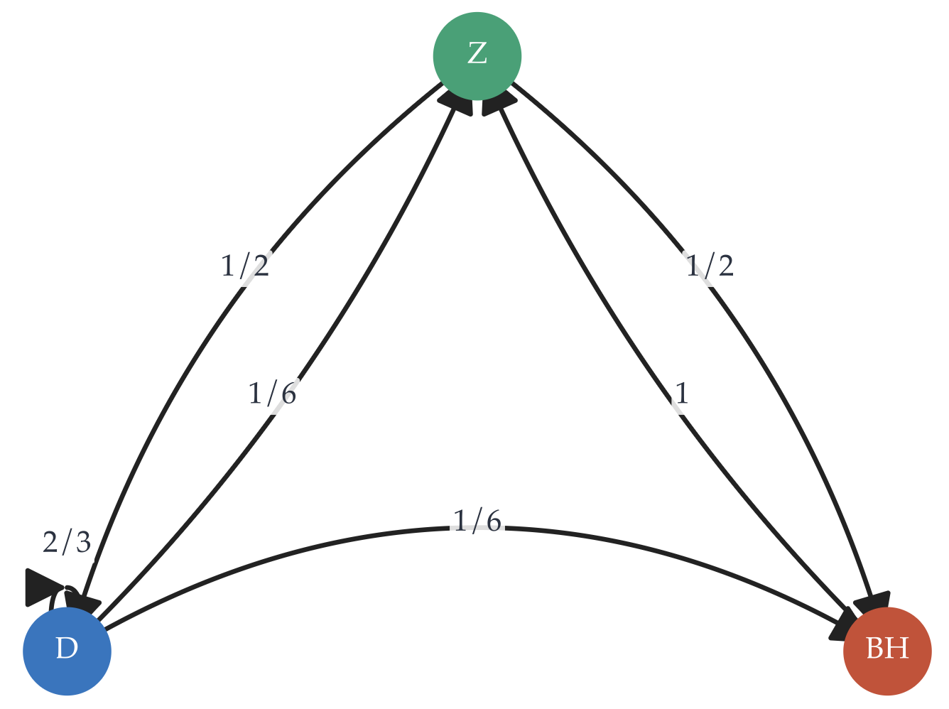
Suppose that each night, a Wolverine moves between three classic Ann Arbor spots: the Diag, Zingerman’s, and the Big House.

  • From the Diag, \(\frac{2}{3}\) of the time it stays at the Diag, \(\frac{1}{6}\) of the time it walks to Zingerman’s, and \(\frac{1}{6}\) of the time it walks to the Big House.

  • From the Big House, it always walks to Zingerman’s.

  • From Zingerman’s, it is equally likely to walk to the Diag or the Big House.

a)

Draw a state diagram for this Markov chain. Make sure to clearly label the edges with their transition probabilities. (For help, see Chapter 9.3.)

Solution
image
b)

Find the adjacency matrix, \(A\), of this Markov chain.

Solution

\(A = \begin{bmatrix} p(D \rightarrow D) & p(B \rightarrow D) & p(Z \rightarrow D) \\ p(D \rightarrow B) & p(B \rightarrow B) & p(Z \rightarrow B) \\ p(D \rightarrow Z) & p(B \rightarrow Z) & p(Z \rightarrow Z) \end{bmatrix} = \begin{bmatrix}2/3 & 0 & 1/2 \\ 1/6 & 0 & 1/2 \\ 1/6 & 1 & 0\end{bmatrix}\)

Let the Diag be state 1, so the first column corresponds to movement from the Diag. The second column corresponds to movement from the Big House, and the third column corresponds to movement from Zingerman’s.

c)

Show that the long-run distribution of the Wolverine’s locations is \(\begin{bmatrix} p(\text{Diag}) \\ p(\text{Big House}) \\ p(\text{Zingerman’s}) \end{bmatrix} = \begin{bmatrix} 6/13 \\ 3/13 \\ 4/13 \end{bmatrix}\). Hint: Do this by finding the eigenvector of \(A\) corresponding to the eigenvalue 1. Since there are infinitely many such eigenvectors, find the one that satisfies the constraint that the components sum to 1.

Solution

We can find the eigenvector corresponding to \(\lambda = 1\) by finding a basis for \(\text{nullsp}(A - \lambda I)\):

$$ \text{nullsp}(A - I) = \text{nullsp}\left(\begin{bmatrix} -1/3 & 0 & 1/2 \\\\ 1/6 & -1 & 1/2 \\\\ 1/6 & 1 & -1 \end{bmatrix}\right)= \text{span}\left(\begin{bmatrix}6 \\\\ 3 \\\\ 4\end{bmatrix}\right) $$

Dividing \(\begin{bmatrix}6 \\ 3 \\ 4\end{bmatrix}\) by the sum of its components, 13, gives us the long-run distribution.

d)

Open a new Jupyter Notebook or interactive Python session in the Terminal. In it, run:

import numpy as np
A = np.array(...) # Replace with the adjacency matrix you found in b)
eigvals, eigvecs = np.linalg.eig(A)

Now, if you run eigvals, you should see

array([ 1.        ,  0.36037961, -0.69371294])

If you run eigvecs[:, 0] to access the eigenvector corresponding to the first eigenvalue in the array above, you should see

array([0.76822128, 0.38411064, 0.51214752])

This is not the eigenvector you found in the previous part. Why not? What did it return, and what expression can you run in code to find the exact answer you found in the previous part?

Solution

np.linalg.eig returns eigenvectors that are unit vectors. Since there are infinitely many eigenvectors in any one direction, a unit eigenvector is the one it chooses to return. To find the eigenvector with a sum of 1, run

eigvecs[:, 0] / np.sum(eigvecs[:, 0])

e)

Run both of the following commands:

np.linalg.matrix_power(A, 20) @ np.array([[1/3], [1/3], [1/3]])
np.linalg.matrix_power(A, 21) @ np.array([[1/3], [1/3], [1/3]])

What do you see? Why?

Solution

The resulting vectors are the same as the long-run distribution from part c) because it’s the eigenvector for the eigenvalue 1, the dominant eigenvalue of the adjacency matrix. Let’s show why it’s converging towards that eigenvector more concretely:

$$ \lambda_1 = 1, \lambda_2 = 0.36, \lambda_3 = -0.69, \vec x = \begin{bmatrix} 1/3 & 1/3 & 1/3 \end{bmatrix}^T $$

All of \(A\)’s eigenvectors, \(\vec v_1, \vec v_2, \text{and } \vec v_3\) are linearly independent, so \(\vec x=c_1\vec v_1 + c_2\vec v_2 + c_3\vec v_3\) for some constants \(c_1, c_2, c_3\).

$$ \begin{align*} A^k\vec x &= A^k(c_1\vec v_1 + c_2\vec v_2 + c_3\vec v_3) \\\\&= c_1A^k\vec v_1 + c_2A^k\vec v_2 + c_3A^k\vec v_3 \\\\&= c_1\lambda_1^k\vec v_1 + c_2\lambda_2^k\vec v_2 + c_3\lambda_3^k\vec v_3 \\\\&= c_1\lambda_1^k\vec v_1 \end{align*} $$

As \(k \rightarrow \infty\), \(\lambda_2^k\) and \(\lambda_3^k\) will both approach 0 because their magnitudes are less than 1, while \(\lambda_1^k\) stays at 1. This leaves us with the eigenvector for \(\lambda_1\).

f)

Now, consider the adjacency matrix

$$ B = \begin{bmatrix} 0 & 0 & 1/2 \\\\ 0 & 0 & 1/2 \\\\ 1 & 1 & 0 \end{bmatrix} $$

Using numpy, find the eigenvalues of \(B\). Then, run all of the following commands:

np.linalg.matrix_power(B, 20) @ np.array([[1/3], [1/3], [1/3]])
np.linalg.matrix_power(B, 21) @ np.array([[1/3], [1/3], [1/3]])
np.linalg.matrix_power(B, 22) @ np.array([[1/3], [1/3], [1/3]])
np.linalg.matrix_power(B, 23) @ np.array([[1/3], [1/3], [1/3]])

This Markov chain appears not to converge. Why not? Relate your answer to the discussion of “the dominant eigenvalue” in Chapter 9.3.

Solution

The eigenvalues of \(B\) are \(\lambda_1 = -1, \lambda_2 = 0, \lambda_3 = 1\). Let’s take a closer look at what happens when we apply the same idea from part e):

$$ \begin{align*} A^k\vec x &= A^k(c_1\vec v_1 + c_2\vec v_2 + c_3\vec v_3) \\\\&= c_1A^k\vec v_1 + c_2A^k\vec v_2 + c_3A^k\vec v_3 \\\\&= c_1\lambda_1^k\vec v_1 + c_3\lambda_3^k\vec v_3 \\\\ \\\\\text{if }k \text{ is even}, &= c_1\lambda_1^k\vec v_1 + c_3\lambda_3^k\vec v_3 \\\\ \text{if }k \text{ is odd}, &= c_1\lambda_1^k\vec v_1 - c_3\lambda_3^k\vec v_3 \end{align*} $$

There are 2 eigenvalues with magnitude 1, and one of them is negative. As \(k \rightarrow \infty\), the result of \(A^k\vec x\) will bounce between two different vectors.


Activity 4: Symmetric Matrices

Suppose \(A\) is a symmetric \(n \times n\) matrix, meaning \(A = A^T\). Symmetric matrices have a special property, described by the spectral theorem: the eigenvectors corresponding to different eigenvalues are orthogonal. Below, we provide a proof of this fact.

1. Let \(\vec v_i\) be an eigenvector of \(A\) with eigenvalue \(\lambda_i\), so \(A \vec v_i = \lambda_i \vec v_i\).

2. Let \(\vec v_j\) be an eigenvector of \(A\) with eigenvalue \(\lambda_j\), where \(\lambda_i \neq \lambda_j\), so \(A \vec v_j = \lambda_j \vec v_j\).

3. The dot product of \(\vec v_i\) and \(A \vec v_j\) is \(\vec v_i \cdot (A \vec v_j) = \vec v_i \cdot (\lambda_j \vec v_j) = \lambda_j (\vec v_i \cdot \vec v_j)\).

4. But also, \(\vec v_i \cdot (A \vec v_j) = \vec v_i^T A \vec v_j = \vec v_i^T A^T \vec v_j = (A \vec v_i)^T \vec v_j = \lambda_i \vec v_i^T \vec v_j = \lambda_i (\vec v_i \cdot \vec v_j)\).

5. The final expressions in both cases are equal, so \(\lambda_j (\vec v_i \cdot \vec v_j) = \lambda_i (\vec v_i \cdot \vec v_j)\).

6. Equivalently, \((\lambda_j - \lambda_i) (\vec v_i \cdot \vec v_j) = 0\). But since \(\lambda_i \neq \lambda_j\), we must have \(\vec v_i \cdot \vec v_j = 0\).

a)

In which line did we use the fact that \(A\) is symmetric? Select the line below, and then in that line, circle the specific part of the equation that uses the fact that \(A = A^T\).

1 2 3 4 5 6
Solution
1 2 3 4 5 6

Line 4 is the only line that uses the fact that \(A = A^T\), but it’s the most important line in the proof. Specifically, here’s where we used that fact:

$$ \vec v_i^T A \vec v_j = \vec v_i^T A^T \vec v_j $$

By using \(A = A^T\) here, we were able to write \(\vec v_i \cdot (A \vec v_j)\) as \(\vec v_i^T A^T \vec v_j = (A \vec v_i) \cdot \vec v_j\), which was key to our final expression.

b)

The spectral theorem states that any symmetric \(n \times n\) matrix \(A\) can be diagonalized by an orthogonal matrix \(Q\) through

$$ A = Q \Lambda Q^T $$

Explain how this relates to the “regular” diagonalization \(A = V \Lambda V^{-1}\). Why does the equation above contain \(Q^T\) instead of \(Q^{-1}\)?

Solution

A standard (not necessarily symmetric) matrix \(A\) that is diagonalizable can be written as

$$ A = V \Lambda V^{-1} $$

If \(A\) is symmetric and can be written \(A = Q \Lambda Q^T\), then the fact that we have \(Q^T\) instead of \(Q^{-1}\) stems from the fact that orthogonal matrices satisfy \(Q^T = Q^{-1}\). This comes from the fact that \(Q^TQ = QQ^T = I\). Transposes are easier to compute than inverses, and easier to interpret, too: if \(Q\) is a rotation, then \(Q^T\) is the inverse rotation, i.e. a rotation by the opposite amount.

c)

Symmetric matrices play a big role in solving optimization problems in machine learning. You’ll get a taste of this in Homework 10, Problem 6, which discusses ridge regression and regularization, ideas that we use to make sure that our models are not overfitting to training data.

Here, we’ll prove a related fact: if \(A\) is an \(n \times n\) symmetric matrix and all of its eigenvalues are non-negative, then \(A\) is positive semidefinite. A symmetric matrix \(A\) is positive semidefinite if and only if \(\boxed{\vec v^T A \vec v \geq 0}\) for all \(\vec v \in \mathbb{R}^n\). One interpretation: this means the quadratic form \(f(\vec v) = \vec v^T A \vec v\) is always greater than or equal to 0, no matter what \(\vec v\) is.

Let’s work through the proof step-by-step: we will do some of it for you, and you’ll complete the rest. (To be precise, we’re only proving one direction of the “if and only if” statement; the other direction is in Homework 10!) First, since \(A\) is symmetric, the spectral theorem tells us that \(A\) can be written as

$$ A = Q \Lambda Q^T $$

where \(Q\) is an orthogonal matrix and \(\Lambda\) is a diagonal matrix with the eigenvalues of \(A\) on the diagonal. This is the eigenvector decomposition of \(A\).

On top of that, suppose that all of \(A\)’s eigenvalues, \(\lambda_1, \lambda_2, \ldots, \lambda_n\), are non-negative.

Now, let \(\vec v\) be some arbitrary vector (not necessarily an eigenvector of \(A\)) in \(\mathbb{R}^n\). Then, eventually we need to show that \(\vec v^T A \vec v \geq 0\), regardless of what \(\vec v\) is. Let’s start by expanding \(\vec v^T A \vec v\) using the fact that \(A = Q \Lambda Q^T\).

$$ \vec v^T A \vec v = \vec v^T (Q \Lambda Q^T) \vec v = (\vec v^T Q) \Lambda (Q^T \vec v) $$

Suppose that \(\vec y = Q^T \vec v\). Then, \(\vec y^T = (Q^T \vec v)^T = \vec v^T Q\). This seems like an arbitrary maneuver, but it will be useful in a moment.

$$ \begin{align*} \vec v^T A \vec v &= \vec y^T \Lambda \vec y =\begin{bmatrix} y_1 & y_2 & \ldots & y_n \end{bmatrix} \begin{bmatrix} \lambda_1 & 0 & \ldots & 0 \\\\ 0 & \lambda_2 & \ldots & 0 \\\\ \vdots & \vdots & \ddots & \vdots \\\\ 0 & 0 & \ldots & \lambda_n \end{bmatrix} \begin{bmatrix} y_1 \\\\ y_2 \\\\ \vdots \\\\ y_n \end{bmatrix} \end{align*} $$

Your job is to complete the rest of the proof. Show that if \(A\) is an \(n \times n\) symmetric matrix and all of its eigenvalues are non-negative, then \(\vec v^T A \vec v \geq 0\) for all \(\vec v \in \mathbb{R}^n\).

Solution
$$ \begin{align*} \vec v^T A \vec v &= \vec y^T \Lambda \vec y \\\\ &= \begin{bmatrix} y_1 & y_2 & \ldots & y_n \end{bmatrix} \begin{bmatrix} \lambda_1 & 0 & \ldots & 0 \\\\ 0 & \lambda_2 & \ldots & 0 \\\\ \vdots & \vdots & \ddots & \vdots \\\\ 0 & 0 & \ldots & \lambda_n \end{bmatrix} \begin{bmatrix} y_1 \\\\ y_2 \\\\ \vdots \\\\ y_n \end{bmatrix} \\\\ &= \begin{bmatrix} y_1 & y_2 & \ldots & y_n \end{bmatrix} \begin{bmatrix} \lambda_1 y_1 \\\\ \lambda_2 y_2 \\\\ \vdots \\\\ \lambda_n y_n \end{bmatrix} \\\\ &= \sum_{i=1}^n \lambda_i y_i^2 \end{align*} $$

Remember that none of the \(\lambda_i\)’s are negative. So, each term \(\lambda_i y_i^2\) is non-negative too, meaning the entire sum \(\sum_{i=1}^n \lambda_i y_i^2\) is non-negative. What we’ve shown is that if \(\vec v\) is any vector in \(\mathbb{R}^n\), then \(\vec v^T A \vec v\) ends up being a sum of this form, which is always non-negative, so \(\vec v^T A \vec v \geq 0\), and thus \(A\) is positive semidefinite.

Activity 5: More Practice (Optional)

Let \(A\) be a \(3 \times 3\) with:

  • eigenvalue \(\lambda_1 = 3\) with eigenvector \(\vec v_1 = \begin{bmatrix} 2 \\ 0 \\ 1 \end{bmatrix}\).

  • eigenvalue \(\lambda_2 = -2\) with the 2-dimensional eigenspace: \(\text{span}\left(\begin{bmatrix} 1 \\ 1 \\ 0 \end{bmatrix}, \begin{bmatrix} 0 \\ 1 \\ 2 \end{bmatrix}\right)\).

a)

Find \(A\). Feel free to use numpy to find an inverse for you and verify your answer.

Solution

\(A = \begin{bmatrix} 0.5 & -2.5 & 5 \\ 0 & -2 & 0 \\ 1.25 & -1.25 & 0.5 \end{bmatrix}\).

The eigenvector decomposition of \(A\) is \(A = V \Lambda V^{-1}\), where \(V\) is the matrix whose columns are the eigenvectors of \(A\) and \(\Lambda\) is the diagonal matrix with the eigenvalues of \(A\) on the diagonal, arranged in the same order as the eigenvectors in \(V\). We know that \(\lambda_1 = 3\) with eigenvector \(\vec v_1 = \begin{bmatrix} 2 \\ 0 \\ 1 \end{bmatrix}\) and that \(\lambda_2 = \lambda_3 = -2\) with eigenvectors \(\vec v_2 = \begin{bmatrix} 1 \\ 1 \\ 0 \end{bmatrix}\) and \(\vec v_3 = \begin{bmatrix} 0 \\ 1 \\ 2 \end{bmatrix}\). Placing this information into \(V\) and \(\Lambda\) gives us

$$ V = \begin{bmatrix} 2 & 1 & 0 \\\\ 0 & 1 & 2 \\\\ 1 & 0 & 1 \end{bmatrix}, \quad \Lambda = \begin{bmatrix} 3 & 0 & 0 \\\\ 0 & -2 & 0 \\\\ 0 & 0 & -2 \end{bmatrix} $$

So,

$$ A = V \Lambda V^{-1} = \begin{bmatrix} 2 & 1 & 0 \\\\ 0 & 1 & 2 \\\\ 1 & 0 & 1 \end{bmatrix} \begin{bmatrix} 3 & 0 & 0 \\\\ 0 & -2 & 0 \\\\ 0 & 0 & -2 \end{bmatrix} \left(\begin{bmatrix} 2 & 1 & 0 \\\\ 0 & 1 & 2 \\\\ 1 & 0 & 1 \end{bmatrix}\right)^{-1} $$

A bit of help from numpy shows that \(A = \begin{bmatrix} 0.5 & -2.5 & 5 \\ 0 & -2 & 0 \\ 1.25 & -1.25 & 0.5 \end{bmatrix}\).

>>> V = np.array([
    [2, 1, 0],
    [0, 1, 2],
    [1, 0, 1]
])
>>> V @ np.diag([3, -2, -2]) @ np.linalg.inv(V)
array([[ 0.5 , -2.5 ,  5.  ],
       [ 0.  , -2.  ,  0.  ],
       [ 1.25, -1.25,  0.5 ]])
b)

Let \(V\) be the matrix whose columns are the eigenvectors of \(A\) and \(\Lambda\) be the diagonal matrix with the eigenvalues of \(A\) on the diagonal. In terms of \(V\) and \(\Lambda\), what is \(A^{8}\)?

Solution

\(A^8 = V \Lambda^8 V^{-1}\).

This comes from the fact that \(A = V \Lambda V^{-1}\), so

$$ A^8 = V \Lambda (V^{-1} V) \Lambda (V^{-1} V) \cdots \Lambda V^{-1} = V \Lambda^8 V^{-1} $$

The sequential multiplication of \(V^{-1}\) with \(V\) cancels out, and we stack together 8 copies of \(\Lambda\).

Since \(\Lambda\) is a diagonal matrix, we can raise each diagonal element to the 8th power.

$$ \Lambda^8 = \begin{bmatrix} 3^8 & 0 & 0 \\\\ 0 & (-2)^8 & 0 \\\\ 0 & 0 & (-2)^8 \end{bmatrix} $$

So, \(A^8 = V \begin{bmatrix} 3^8 & 0 & 0 \\ 0 & (-2)^8 & 0 \\ 0 & 0 & (-2)^8 \end{bmatrix} V^{-1}\).

c)

Suppose \(\vec x \in \mathbb{R}^3\) is some vector. As \(k \to \infty\), what does \(A^k \vec x\) approach? Explain your answer in English.

Solution

As \(k \to \infty\), \(A^k \vec x\) approaches the eigenvector corresponding to \(\lambda_1 = 3\) (the dominant eigenvalue), so some scalar multiple of \(\vec v_1 = \begin{bmatrix} 2 \\ 0 \\ 1 \end{bmatrix}\).

Remember that \(A^k = V \Lambda^k V^{-1}\). As \(k\) increases, the diagonal entries of \(\Lambda^k\) — \(3^k, (-2)^k, (-2)^k\) — all grow exponentially larger, but \(3^k\) grows faster than \((-2)^k\). So, the contribution of the second and third eigenvectors to \(A^k \vec x\) diminishes, and \(A^k \vec x\) approaches a scalar multiple of \(\vec v_1\).

To be clear, the numbers in \(A^k \vec x\) will approach infinity; it’s the direction of \(A^k \vec x\) that approaches the direction of \(\vec v_1\). Simulate this in numpy to see for yourself!

>>> x = np.array([[1], [1], [1]])
>>> A = np.array([
    [0.5, -2.5, 5],
    [0, -2, 0],
    [1.25, -1.25, 0.5]
])
>>> x_k = np.linalg.matrix_power(A, 50) @ x
>>> x_k # Massive numbers!
array([[7.17897988e+23],
       [1.12589991e+15],
       [3.58948994e+23]])
>>> x_k / np.linalg.norm(x_k) # Unit vector makes numbers smaller.
array([[8.94427191e-01],
       [1.40275570e-09],
       [4.47213596e-01]])
# Notice that the unit vector is roughly [2, 0, 1] multiplied by a scalar.